To any coffee-lover, waiting in line for your morning fix can already feel like a project. So to make less of a project for myself in the future, I wanted to investigate my favorite café spot’s busiest times to figure out how long it typically takes from the time I walk through the door to the time I pay for my coffee. But with so many other caffeine-cravers lining up all over the Terrace, I was also a bit curious to know what the morning rush hour looked like from their perspective, too.
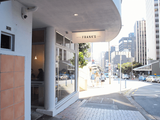
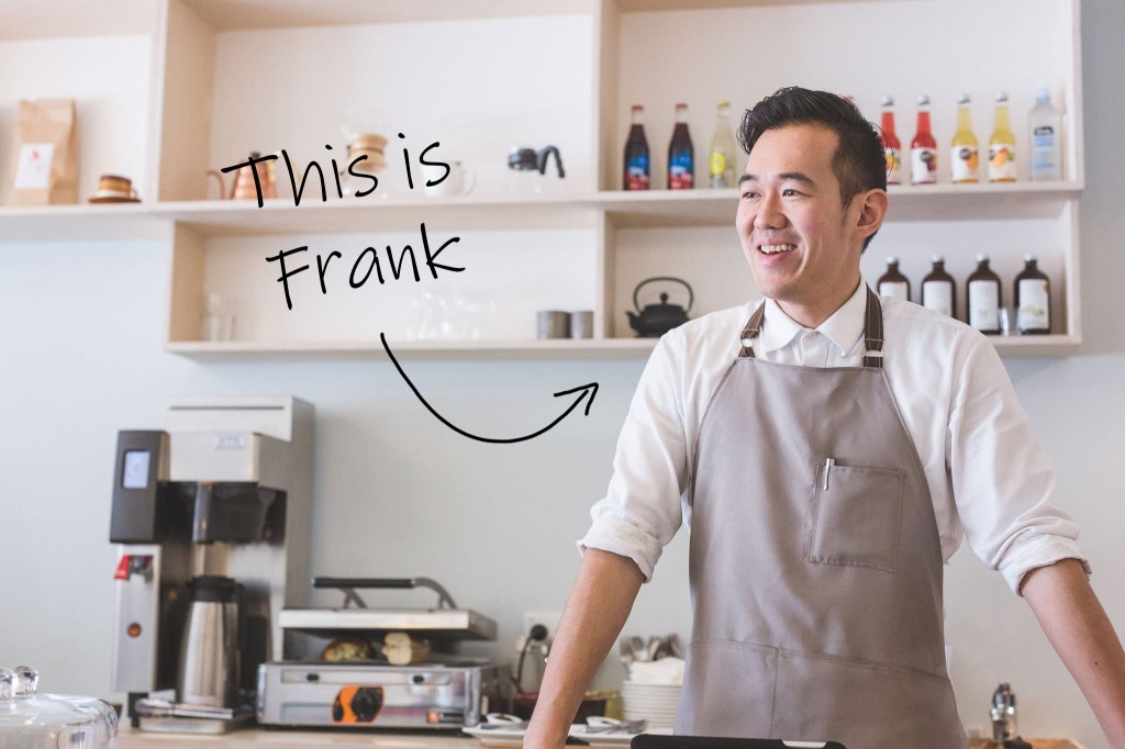
Frank’s Café is a locally run business that can be found here on the Wellington Terrace. It’s a good spot for great coffee and can regularly be found bustling with customers. After getting permission from Frank himself to record some of this flow of activity, I performed an analysis on the data to deduce the nature of the line and service distributions the system experiences during their most populous hours. Then finally, I simulated these behaviors in Python to gather some of the system’s measurements. Frank shared that his busiest times tended to be Thursday and Friday mornings between 8-10am (unsurprisingly, their ‘donut-selling days‘), so that’s where I began.
If you haven’t tried Frank’s coffee and bi-weekly donuts yet, I highly suggest clearing your Thursday or Friday morning schedule to pick this article back up then and there. Or, you can read this first so that you’re prepared to experience their busiest time of day and the average 119 seconds from the time you walk through Frank’s door to the time you order your ‘cuppa (which by the way, is pretty impressive for a rush hour wait time – good job, Frank’s team!). But how do I know that the expected time spent in their queue during rush hour is between 42-196 sec and averages around 119 sec, you ask? Did I just simply time how long it takes to pass through the queue, order, and pay? Well, yes and no. I timed the process, yes, but many, many times over and probably not quite the way you’re thinking. I also complicated things almost unnecessarily with some distributional analyses and simulations to create a much more robust approximation of Thursday and Friday coffee & donuts through Frank’s eyes!
Getting the Data from Frank’s
(*No one was video or audio recorded for this process! Events were recorded with the press of a laptop key, ‘A’, ‘S’, or ‘D’ using a special python script that you can find here, along with all the other scripts for this project.)
Customer Event Recording Sessions:
- Thursday 18th March (between 8-10am)
- Friday 19th March (between 8-10am)
- Thursday 25th March (between 8-10am)
- Friday 26th March (between 8-10am)
The recording process itself was rather straight forward…
- When someone walks into the shop; they’re considered an arrival. I press ‘A‘ on my keyboard.
- When someone begins to speak their order to the cashier; that’s considered the start of service. I press ‘S‘ on my keyboard.
- When someone pays for their order; that’s considered the end of service (departure). I press ‘D‘ on my keyboard.
Flash forward two weeks, twelve coffees, four friends and 937 unique event recordings later, and we’re looking at a rather messy dataset consisting of: 338 arrivals, 297 beginnings of service, and 302 ends-of-service (which I’ll now start referring to as ‘departures’).
We now have our single-server system and a whole bunch of data points. The next step is cleaning the data and balancing our classes. I don’t want to have to impute too many values because the number of instances already rather small, so instead we level the data off to 302 arrivals, services, and departures. We then compute the differences between the three different types of events we observed:
- Time between two arrivals (the ‘interarrival time’)
- Time between two service events (the ‘service time’)
- Time between an arrival and service (the time spent waiting in the queue)
What does each of these differences tell us? Respectively, they tell us: (1) the amount of time that passes between two customers walking through the door, (2) the amount of time someone spends waiting, ordering and paying at the till, and lastly (3) the amount of time spent waiting in line to order.
Let’s Get to Fitting!
The donuts may not have help my pants fit better, but they certainly helped me fit the data to their theoretical distributions by bringing enough customers through the door to form a queue! Speaking of queues, now is a good time to talk about some fundamentals of queueing systems so that we can continue studying Frank’s Café. What is a queueing system? It is anything that requires customers to wait in line for a service. You are probably already very familiar with waiting in queues yourself, and though you may not often think about how you wait for a service – whether it’s food, shopping, or something else – I can guarantee that if you’re queueing at a commercial business, someone has thought about how you and all of their other customers wait in line.
When we want to take measurements of a queueing system, such as the average time spent in the system or the average number of people in the queue, there are a few things that need to be mathematically established; and the first, most important condition is that we have what we refer to as a ‘steady state distribution’. That is, we can’t have more customers entering the system than leaving it over the specified time period, otherwise we accrue system build-up. The other helpful thing to know is that there is a fancy formula called Little’s Law. This formula becomes very important later, but for now just know that Little’s Law is an equation which gives us information such as the ‘average time in the queue’, ‘average number of customers in the queue’, ‘server utilization’, etc. But for us to be able to use it, we can’t have more customers coming into the system than going out. That is to say, we can’t have customers arriving more frequently than than our server can get them through service!
How can we be sure that we have a steady state system so that we’re able to measure it with this mysterious Little’s Law? First we go back to our data and take the mean times between arrivals and services. These two values are often represented as ‘E(A)‘ and ‘E(S)‘ respectively and they refer to the mean – a point-value estimation. In this case, we want the expected time between arrivals (E(A)) and the expected time between services (E(S)). To decide whether or not we’re dealing steady state system, both of these expected values must be expressed in the same time units so that we can compare them directly.
In mathematical notation, we would introduce two new parameters called the interarrival rate, λ (“lambda”), and the service rate, μ (“mu”). To turn our expected times into rates, we just put 1/E(A) or 1/E(S). For this system, I measured the time in seconds. So to get the number of customer arrivals per second, we use 1 (second) over the mean arrival time (and then apply the same principle to service times). At Frank’s café during the observed period, the mean time between arrivals was 70.64sec and the mean time between services was 72.75sec. Therefore λ = 0.0142, μ = 0.0137. Additionally, our interarrival and service rates are already expressed in matching time units, so we can now make our next comparison.

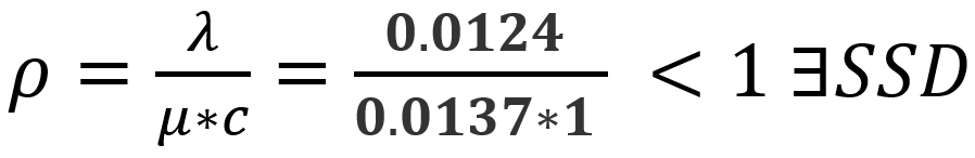
As I mentioned earlier, to have a steady state system we cannot have customers arriving at a rate greater than the rate at which they’re being served (otherwise the system gets backed up with customers). To test if this is the case for our observations, we use a handy formula referred to as the ‘traffic equation’. This traffic equation tells us whether or not the system is in steady state (i.e. if λ/μ < 1, then steady state exists). The traffic equation is represented as ρ (“rho”), a parameter referred to as the ‘traffic intensity’. When ρ < 1, we say that steady state exists.
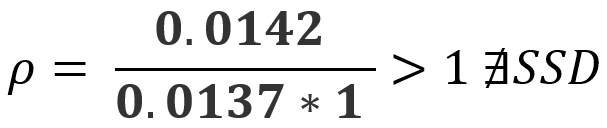
Don’t worry that sneaky ‘c‘ is just our number of servers; which at Frank’s for the observation period was just one brave, lone cashier. But, if we look a bit more closely we can see that we have a problem λ > μ, and that series of symbols ‘∄SSD‘ is unfortunately how we express “steady state does not exist“. So what do we do? We put on our empirical thinking caps!
Because this was an experiment in which we collected raw data, we can use the central limit theorem to figure out our 95% confidence interval for the mean interarrival time and hope that one of those values allow us to establish steady state. Because of some of the tricky nuances of simulating Frank’s queuing system later on, we need to approach this problem by ever-so-slightly perturbing our interarrival data to give us λ < μ within the interval in which we can be 95% confident that the value of E(A) lies.
With all this math it’s been a while since we’ve seen a real person, so let me share the formula for a confidence interval with a warm, friendly barista from Frank’s.

That’s Manuel, and I have his permission to show you the back of his head while I share this formula:
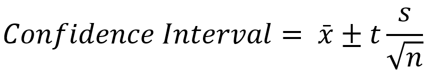
In this formula (underpinned by the central limit theorem), s is the standard deviation of the sample, n is the sample size, s/√n is the standard error (a measure of the expected spread of the means), t is a value determined by the sample size and chosen level of confidence, and t * s/√n is the margin of error, which is finally added or subtracted to x̄, the sample mean. Using this, we can calculate our 95% confidence interval for the interarrival time as [60.34, 80.92]. Which is to say: we can be certain that our mean interarrival time will fall between 60.34 and 80.92 seconds with a 95% probability. There’s also something interesting to point out from this formula that helps us understand why small sample sizes tend to have wider confidence intervals (which isn’t a good thing): the √n is reflective of the concept that more information we have, the less new information we get from +1 observation in the sample. Mathematically, this is how we prove and achieve narrower confidence intervals for larger sample sizes.
But don’t get distracted! This is all just an intermediate, compensatory step. Back to the task at hand – we need to disrupt those interarrival times to artificially nudge our mean farther to the right and achieve a measurable steady state system.
To do this, I add interarrival times to the dataset that represent fake (imputed) customers whose interarrival times are between the upper bound of the confidence interval (80.92 sec) and the maximum interarrival time observed in this system (522.63 sec), such that (80.92 < x < 522.63). Adding anywhere between 5 -8 new customers to our set of 302 tends to do the trick. And now ladies, gentlemen, and friends beyond the binary, we can see that this steady state exists, and be 95% confident that this is still within our observed system!

Phew! We finally obtained data for a system that we’re sure we can observe. Now it’s time to figure out what the best-fitting distributions for the interarrival and service times are. For efficiency, I tested the fit of my data against 89 different possible distributions, using the Sum of Squared Estimate of Errors (SSE) as a goodness-of-fit metric. The sum of squared estimate of errors is the sum of deviational errors between the empirical and predicted value. If that sentence is confusing to you and you’d like to learn more about this step, you can do so here. In the simplest terms, the smaller the SSE-value, the tighter the model is fit to the data (which is a good thing, as that means our model is closer to representing the actual system).


In doing this, I discovered that the best-fit distribution to interarrival times was Fatigue Life (SSE = 0.0052), and for service times the best-fit distribution was Log Laplace (SSE = 0.0021):


Simulating Frank’s Coffee Service with SimPy
Now that we have our best-fit distributions and our interarrival and service rates, we can run some simulations and actually measure this system. The following code is written in Python; you can run it online in Jupyter Notebooks or any other Python-compatible IDE of your choice. And again, you can find this example and all the other code for this project here. You’ll need to install SimPy or SimPy Classic to be able to follow along!
#Uncomment these lines to install SimPy Classic
#import sys
#!{sys.executable} -m pip install SimPyClassic

"""M1: Observed System represented as M/M/1 Queueing System"""
from SimPy.Simulation import *
import random
import numpy
import math

## Useful extras ----------
def conf(L):
    """confidence interval"""
    lower = numpy.mean(L) - 1.96*numpy.std(L)/math.sqrt(len(L))
    upper = numpy.mean(L) + 1.96*numpy.std(L)/math.sqrt(len(L))
    return (lower,upper)

## Model ----------
class Source(Process):
    """generate random arrivals"""
    def run(self, N, lamb, mu):
        for i in range(N):
            a = Arrival(str(i))
            activate(a, a.run(mu))
            t = random.expovariate(lamb)
            yield hold, self, t

# Arrival ---------
class Arrival(Process):
    """an arrival"""
    n = 0 # class variable (number in system)

    def run(self, mu):
        # Event: arrival
        Arrival.n += 1 # number in system
        arrivetime = now()

        G.numbermon.observe(Arrival.n)
        if (Arrival.n>0):
            G.busymon.observe(1)
        else:
            G.busymon.observe(0)

        yield request, self, G.server
        # ... waiting in queue for server to be empty (delay) ...
        waitTime = now()-arrivetime
        G.waitmon.observe(waitTime)

        # Event: service begins
        t = random.expovariate(mu)

        yield hold, self, t
        # ... now being served (activity) ...

        # Event: service ends
        yield release, self, G.server # let go of server (takes no simulation time)

        Arrival.n -= 1
        G.numbermon.observe(Arrival.n)
        if (Arrival.n>0):
            G.busymon.observe(1)
        else:
            G.busymon.observe(0)
        delay = now()-arrivetime
        G.delaymon.observe(delay)
        G.servicemon.observe(delay-waitTime)

## Experiment ----------------
allW = []
allL = []
allB = []
allWS= []
allWQ= []
allLS= []
allLQ= []
allLambdaEffective = []

# Values from data analysis
observed_lambda = 1/arrival_mean_upper_CI
observed_mu = 1/service_mean

for k in range(50):
    seed = 123*k
    result = model(c=1, N=10000, lamb=observed_lambda, mu=observed_mu, maxtime=2000000, rvseed=seed)
    allW.append(result[0])
    allL.append(result[1])
    allB.append(result[2])
    allWQ.append(result[3])
    allWS.append(result[4])
    allLQ.append(result[5])
    allLS.append(result[6])
    allLambdaEffective.append(result[1]/result[0])

print("------------ M1 : M/M/1 System Representation ------------")
What this block of code does:
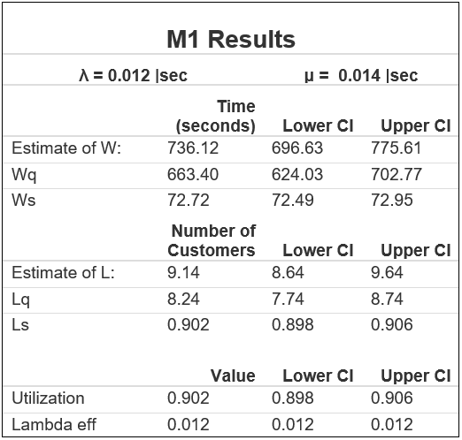
This model assumed that Frank’s Café was an M/M/1 type queueing system, which is Kendall-Lee Notation for a system with identical and independently distributed exponential interarrival and service times, served by one server. Thanks to our adjusted lambda and mu, this period was observable. Of course, its results don’t offer any insight about Frank’s Café as a queueing system because we presumed the distributions to be exponential, but are mindful that the true best-fit interarrival and service times are Fatigue Life and Log Laplace. Still, this simulation is easier to follow than the next two and offers some insight about the range of values that we might expect under different system conditions. For the first time, we have some system measurements to look at:
Interpreting M1 Results
- W = Average time spent in the system = 736 seconds (697, 776) 95% CI
- Wq = Average time spent in the queue = 663 seconds (624, 703) 95% CI
- Ws = Average time spent in service = 72.8 seconds (72.5, 73.0) 95% CI
- L = Average no. of customers in the system = 9.14 customers (8.64, 9.64) 95% CI
- Lq = Average no. of customers in the queue = 8.24 customers (7.74, 8.74) 95% CI
- Ls = Average no. of customers in service = 0.902 customers (0.898, 0.906) 95% CI
- Server Utilisation (p) = 0.902 (0.898, 0.906) 95% CI (*This will always = Ls in the case of one server.)
These results, again, aren’t representative of Frank’s Café but we can practice interpreting the table. L and W are representations of the average number of customers in the system, and average time spent in the system, respectively. They come from Little’s Law – the formula that I mentioned earlier which informs different sorts of averages in queues. Little’s Law states:

Where L = average number of customers in the system, W = average time spent in the system, and λ_eff (“lambda effective”) = N (number of jobs in the system) * T (time in the system) = average arrival rate of jobs entering the system. This is true for any period that defines zero customers in the queue at the beginning and end of observation. When we make T very large (i.e. approach infinity), we are able to use this formula for long-run and steady state systems. This is what a theoretical M/M/1 system looks like, along with each of its performance measures that have been derived from Little’s Law equation:

While the theory behind this is hugely important, it’s a bit beyond the scope of this article, but still – we can now perform a sanity check on the values produced by our M1 simulation:
| Sanity Check (Theoretical) | M1 Results (Simulation) | Within 95% CI? |
| λ = 0.0124 | λ = 0.0124 |  |
| μ = 0.0137 | μ = 0.0137 | |
| ρ = 0.905 | ρ = 0.902 (0.898, 0.906) | |
| W = 769 | W = 736 (697, 776) | |
| L = 9.54 | L = 9.14 (8.64, 9.64) | |
Fantastic! Now we know that our simulation is representing a valid M/M/1 system. Let’s move on to something a bit more sophisticated and accurate to Frank’s system.
We can use our adjusted data to build an empirical model based on the principles of a probability mass function (PMF) and the cumulative density function (CDF) to calculate the area under the distribution. The result of this is a probability distribution for our observed data. Out of all of the models, this one is the one which we would expect to be the closest representation of the real-life system. This is because our predictions are being based directly off of the discrete dataset. Just a word of caution, though: this model can take up to 30min to run, so let’s first have a look at its results:
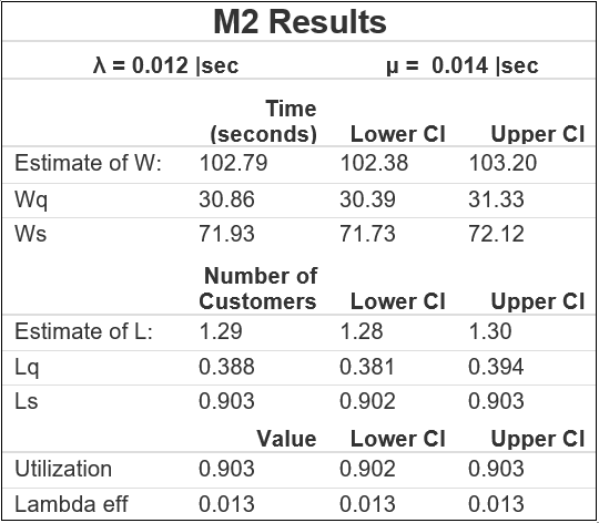
Interpreting M2 Results
- W = Average time spent in the system = 103 seconds (102, 103) 95% CI
- Wq = Average time spent in the queue = 30.8 seconds (30.4, 31.3) 95% CI
- Ws = Average time spent in service = 71.9 seconds (71.7, 72.1) 95% CI
- L = Average no. of customers in the system = 1.29 customers (1.28, 1.30) 95% CI
- Lq = Average no. of customers in the queue = 0.388 customers (0.381, 0.394) 95% CI
- Ls = Average no. of customers in service = 0.903 customers (0.902, 0.903) 95% CI
- Server Utilisation (p) = 0.903 (0.902, 0.903) 95% CI
What’s our sanity check in this case?
Well, we don’t need much to confirm the sanity of our model. It’s clear that the confidence intervals are much more narrow than in our first run because we are no longer basing our estimations on some prescribed probability density function (PDF). Our utility is a value that we would expect (0.903) based on our observed mu and adjusted lambda. The only unique characteristic of this model is our λ_eff, that is our average arrival rate for the entire system, is higher than 0.0124 because it is beginning to converge with our original unadjusted λ. This is expected, though, if you recall that we only slightly perturbed the data to make our system observable – resulting in a relatively minimal affect on the interarrival distribution. This convergence makes the Frank’s Café data a bit trickier to observe and starts to hint at why we’re likely to run into trouble if we simulate this system using the best-fit distribution PDFs in place of the empirical dataset.
Now let’s try the final simulation. We want to use our best-fit distributions (Fatigue Life and Log Laplace) to make universal assumptions about Frank’s Café for the specified interval; this will allow us to account for normal (expected) variation within the system. This step effectively gives our model predictive power to reflect our assumptions onto almost Thursday or Friday mornings at Frank’s. But as I said before, this is where things get a bit tricky. Below are the results obtained for M3:

Interpreting M3 Results
- W = Average time spent in the system = 281 seconds (199, 362) 95% CI
- Wq = Average time spent in the queue = 119 seconds (41.9, 196) 95% CI
- Ws = Average time spent in service = 162 seconds (152, 171) 95% CI
- L = Average no. of customers in the system = 3.61 customers (2.45, 4.77) 95% CI
- Lq = Average no. of customers in the queue = 1.51 customers (0.41, 4.77) 95% CI
- Ls = Average no. of customers in service = 2.10 customers (2.01, 2.19) 95% CI
- Server Utilisation (p) = 0.867 (0.849, 0.884) 95% CI
Because these distributions are very closely fitted to our dataset, perturbing the mean doesn’t really help us conceal that oversized lambda anymore. In fact, you can see the upper bound of the utilisation confidence interval is once again greater than mu (0.014 > 0.0137), thus breaching steady state. The only way that we can compensate for this is to add more servers to the system – 4, to be exact – for a total of 5 servers. This gives us roughly the same system utilization (0.867) as before. Our system is observable thanks to that ‘sneaky c‘ parameter representing our number of servers in our traffic equation, but needing to add more servers indicates that these distributions tend towards non-steady state. For Frank, that means that it’s a good thing rush hour has an end, otherwise customers would be backing up all the way down the Terrace!
Assuming that we did have steady state system with just Frank manning the till though, we learn all types of useful information about our system; we now know that we’ll be waiting in line for at least 42 seconds to get from the door to ordering at the counter, spend anywhere from 152-171 seconds at the counter, and see anywhere between 2-5 other patrons in line.
Of course, it is important to remember that having such a small sample size makes our model very sensitive to anomalous events, but perhaps having even one extra worker on during rush hours could help balance the flow of this system.
And that concludes our investigation! So the next time you’re at Frank’s for Thursday or Friday morning coffee and donuts, don’t be surprised if it happens to take you around 119 seconds to get through the queue. But one thing is for certain; the reward is well worth the wait!
Again, a huge thank you to Frank and his staff for letting us record at the café! Please consider buying a cup from Frank’s the next time you find yourself in the area and craving a coffee or a snack, and remember to support local businesses like Frank’s!