
Background
Model-free reinforcement learning is a class of reinforcement learning methods in which agents learn to make decisions directly from their interactions with the environment without re-training or using a model of the environment’s dynamics.
In MFRL, the agent does not attempt to explicitly learn the transition probabilities P(s′∣s, a) or the reward function R(s,a). Instead, it focuses on learning the value of actions or states from trial-and-error experiences.
There are two broad categories of MFRL methods:
- Policy-based methods which learn the policy pi(a|s) directly (e.g., REINFORCE, PPO), and
- Value-based methods (discussed in this project article), which estimate value functions V_π(s) or action-value functions Q_π(s,a) (e.g., TD Learning, Q-learning, SARSA).
For MFRL through TD Learning, see this project article.
Feeling a little lost? Try reading this project article on policy-based methods first.
Q-Learning
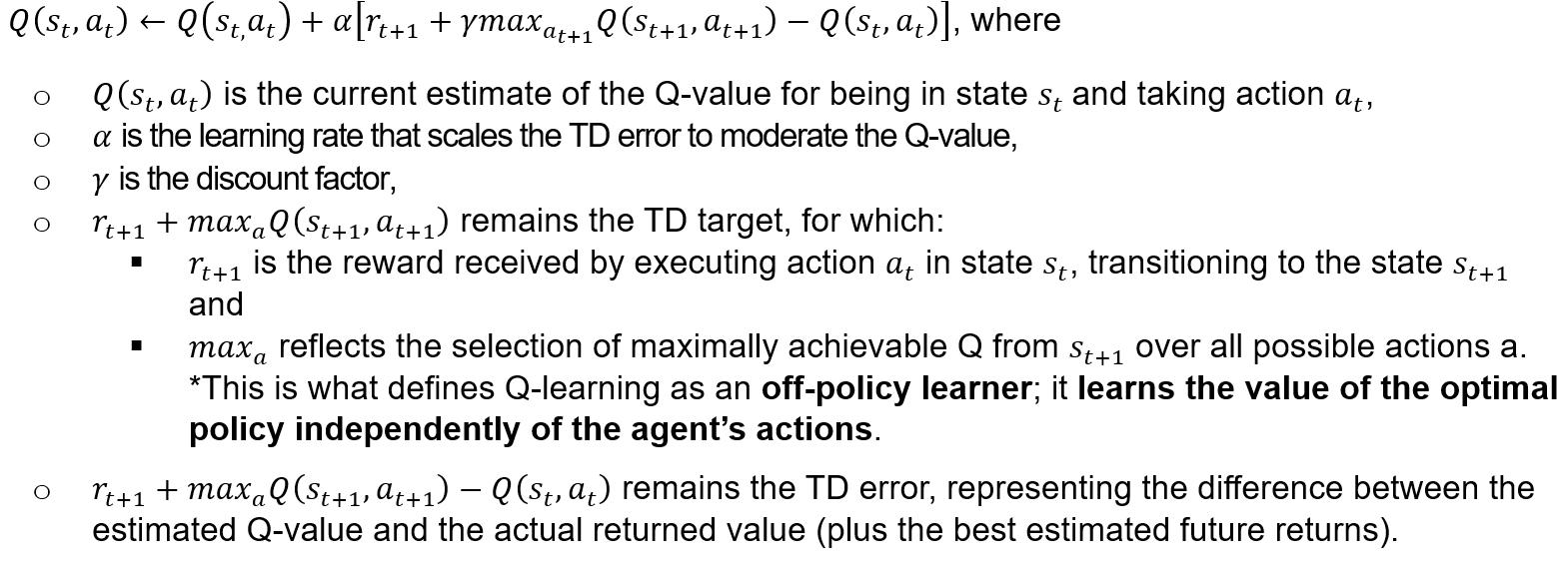
Q-learning is a model-free reinforcement learning algorithm used to find the optimal action-selection policy for a finite MDP. It aims to learn the value of state-action pairs, known as the optimal Q-values, which indicate the expected return of taking a given action in a given state and following the optimal policy thereafter. To do so, we store all the Q-values in a table that we will update at each time step using the Q-learning updating rule:


We begin with the initialisation step, where Q-values for all state-action pairs are initialised using zeros or small random values to facilitate learning.
The learning rate, alpha (α), determines how much new information overrides historical information. A smaller α-value leads to more conservative updates.
The discount factor γ is applied to future rewards. It is used to balance the total value with respect to immediate and future rewards. A higher γ values future rewards more favorably.
The ϵ-greedy action selection strategy is used to encourage (mostly) greedy actions while introducing some randomness for new exploration. The ϵ-greedy action is assigned the value 1-ϵ, where ϵ is the probability assigned to taking a random action in the selected exploration.
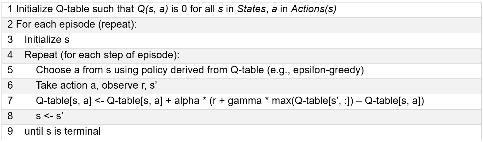
Q-Learning Approach (Reminder)
As a reminder, we apply the same TD(0) principles to a Q-learning update:
Pseudocode:
Toy-box Example: The Frozen Lake (FrozenLake-v1) Environment
FrozenLake-v1 is a standard testing environment in OpenAI Gym. The agent controls the movement of a character in a grid world. Some tiles of the grid are walkable, and others lead to the agent falling into the water. The agent’s goal is to reach the goal tile without falling into the water (OpenAI Gym Library, 2022).

This problem is an example of an MDP.
Loading the Gym & Running the Frozen Lake Simulation:
import numpy as np
import matplotlib.pyplot as plt
import gym
import pandas as pd

env = gym.make('FrozenLake-v1', is_slippery=True)

# problem conditions
num_runs = 5
all_rewards = []

for run in range(num_runs):
    np.random.seed(run)

    # initialize Q-table
    Q_table = np.zeros((env.observation_space.n, env.action_space.n))

    n_episodes = 10000
    max_iter_episode = 100
    exploration_proba = 1  # epislon start = 1
    exploration_decreasing_decay = 0.01
    min_exploration_proba = 0.01
    gamma = 1
    lr = 0.1

    # track rewards per episode
    rewards_per_episode = []

    # iterate over episodes
    for e in range(n_episodes):
        initial_state = env.reset()
        current_state = initial_state[0] if isinstance(initial_state, tuple) else initial_state  # extract state index
        done = False
        total_episode_reward = 0

        for i in range(max_iter_episode):
            if np.random.uniform(0, 1) < exploration_proba:
                action = env.action_space.sample()
            else:
                action = np.argmax(Q_table[current_state, :])

            next_state, reward, done, other_flag, info = env.step(action)  # environment step

            # Update Q-table using the Q-learning iteration
            Q_table[current_state, action] = (1 - lr) * Q_table[current_state, action] + lr * (reward + gamma * np.max(Q_table[next_state, :]))
            total_episode_reward += reward

            if done:
                break

            current_state = next_state

        exploration_proba = max(min_exploration_proba, np.exp(-exploration_decreasing_decay * e))
        rewards_per_episode.append(total_episode_reward)

    all_rewards.append(rewards_per_episode)

# Prepare data (calculate means)
mean_rewards = np.mean(np.array(all_rewards), axis=0)  # average over runs

# Tabulation
data = {
    "Episode Milestone": [(i+1)*1000 for i in range(10)],
    "Mean Episode Reward": [np.mean(mean_rewards[1000*i:1000*(i+1)]) for i in range(10)]
}
df = pd.DataFrame(data)
# index to episode milestones
df.set_index('Episode Milestone', inplace=True)
# float precision format
pd.options.display.float_format = '{:,.4f}'.format
print(df)

# Graph moving average
def moving_average(data, window_size):
    """ Compute moving average using a specific window size """
    return np.convolve(data, np.ones(window_size)/window_size, mode='valid')

window_size = 100  # adjust smoothing
smoothed_rewards = moving_average(mean_rewards, window_size)

plt.figure(figsize=(12, 6))
plt.plot(smoothed_rewards)
plt.title('Learning Performance Over Episodes (Smoothed)')
plt.xlabel(f'Episodes (Averaged every {window_size} episodes)')
plt.ylabel('Average Reward')
plt.grid(True)
plt.show()

# Assuming mean_rewards contains the average rewards per episode
mean_performance = np.mean(mean_rewards)
std_dev_performance = np.std(mean_rewards)
median_performance = np.median(mean_rewards)
min_reward = np.min(mean_rewards)
max_reward = np.max(mean_rewards)

print(f"Average Learning Performance: {mean_performance:.4f}")
print(f"Standard Deviation: {std_dev_performance:.4f}")
print(f"Median Performance: {median_performance:.4f}")
print(f"Minimum Reward Achieved: {min_reward:.4f}")
print(f"Maximum Reward Achieved: {max_reward:.4f}")

# Plotting with annotations
plt.figure(figsize=(12, 6))
plt.plot(smoothed_rewards)
plt.title('Learning Performance Over Episodes (Smoothed)')
plt.xlabel('Episodes (Averaged every 100 episodes)')
plt.ylabel('Average Reward')
plt.axhline(y=mean_performance, color='r', linestyle='-', label=f"Mean Performance: {mean_performance:.4f}")
plt.legend()
plt.grid(True)
plt.show()
Model Results:
Results of running the Q-learning algorithm on the FrozenLake-v1 environment with given parameters (Amine, 2020):

Next, we want to examine the results of running the Q-learning algorithm under the specified conditions (see table above)…
Performance curve of the Q-learned table after 5-independent runs:
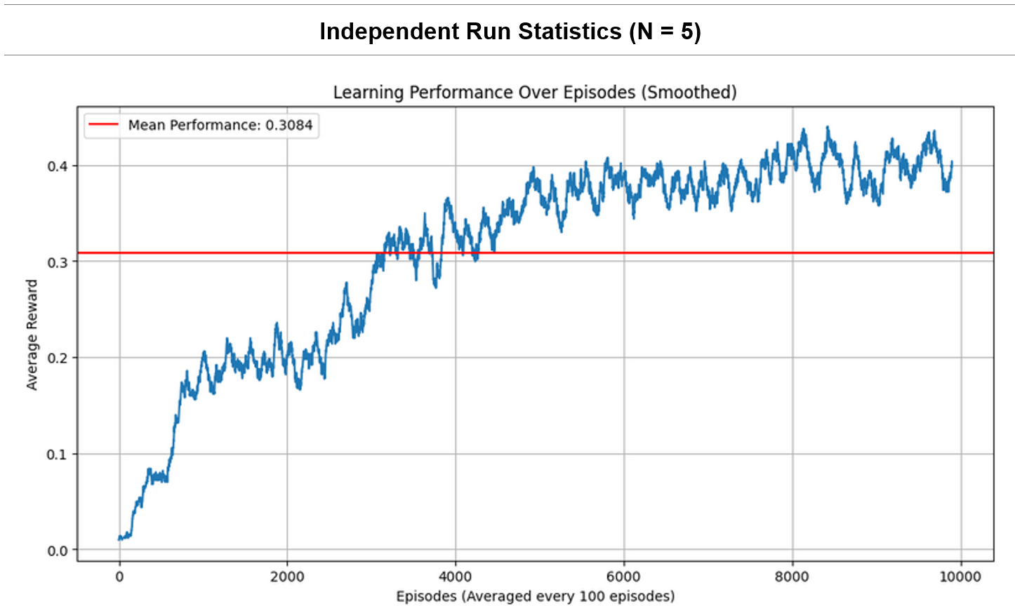
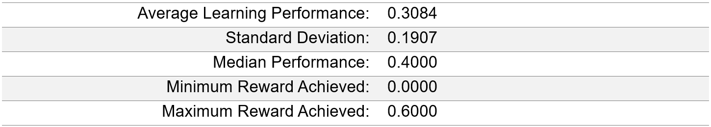
Results Discussion:
There is a significant rise in average reward during the initial learning phase, indicating effective learning and policy improvement. Performance stabilizes with a mean reward of 0.3084, indicating convergence. Despite convergence, the rewards display variability (SD = 0.1907) and fluctuation between a minimum reward of 0.0 and a maximum of 0.6 – likely a consequence of the stochasticity of FrozenLake-v1.
The exploration rate decay is set to allow a gradual shift from exploration to exploitation. As specified by the problem, the exploration rate (ϵ) starts at 1, promoting initial exploration of the state-action space. As ϵ decays, the agent increasingly exploits its accumulated knowledge (i.e., explores less and “acts more greedily”), which correlates with a rise in performance. The exploration rate’s exponential decay ensures that the agent does not stop exploring entirely, even in later episodes.
Overall, Q-learning appears to be an effective approach for the FrozenLake-v1 environment, as demonstrated by consistent improvement and eventual stabilisation in the rewards. The algorithm’s learning and improvement over time is reflected in its increasing performance (smoothed by moving average) on the curve until it converges, thus supporting its suitability for this type of discrete, stochastic problem.
References
Amine, A. (2020). Q-Learning Algorithm: From Explanation to Implementation. Medium. https://towardsdatascience.com/q-learning-algorithm-from-explanation-to-implementation-cdbeda2ea187
Chen, A. (2024). AIML431: Dynamic Programming Lecture Notes. Victoria University of Wellington. https://ecs.wgtn.ac.nz/foswiki/pub/Courses/AIML431_2024T2/LectureSchedule/dp.pdf
Kleijn, B. (2024). Basic Deep Learning Regressor & Gradient Descent and Context: AIML425 [Lecture 3 & 4 Notes]. Master of Artificial Intelligence, Victoria University of Wellington. https://ecs.wgtn.ac.nz/foswiki/pub/Courses/AIML425_2024T2/LectureSchedule/DLintro.pdf
OpenAI Gym Library. (2022). FrozenLake-v0. In Gym Documentation. https://www.gymlibrary.dev/environments/toy_text/frozen_lake/#version-history
