
Background
Model-free reinforcement learning is a class of reinforcement learning methods in which agents learn to make decisions directly from their interactions with the environment without re-training or using a model of the environment’s dynamics.
In MFRL, the agent does not attempt to explicitly learn the transition probabilities P(s′∣s, a) or the reward function R(s,a). Instead, it focuses on learning the value of actions or states from trial-and-error experiences.
There are two broad categories of MFRL methods:
- Policy-based methods which learn the policy pi(a|s) directly (e.g., REINFORCE, PPO), and
- Value-based methods (discussed in this project article), which estimate value functions V_π(s) or action-value functions Q_π(s,a) (e.g., TD Learning, Q-learning, SARSA).
Temporal Difference (TD) Learning
Temporal difference (TD) learning is a value-based, model-free RL method that learns by bootstrapping, i.e., online learning. TD models take the approach of updating estimates based on other learned estimates, rather than waiting for final outcomes (as in Monte Carlo [MC] methods).
TD learning is more common and efficient than MC reinforcement learning because TD methods learn directly from episodes of experiences. Like MC methods, they are model-free with no knowledge of transition models and reward functions. However, unlike MC, they use state transitions to bootstrap their learning. Further, they learn policies from value functions (i.e., Bellman Expectation Equation), as observed in dynamic programming.
In more formal terms, the goal of a TD method is to learn v_pi online from experience under policy pi, where ‘online’ describes a model capable of simultaneously sampling and learning a v-function.
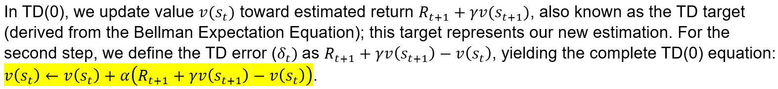
The simplest TD learning algorithm is TD(0):
Feeling a little lost? Try reading this project article first.
TD(0) Learning Example
In this example, we are presented with the transition sample (Table 1, below):

Applying the TD(0) principles to a Q-learning update:
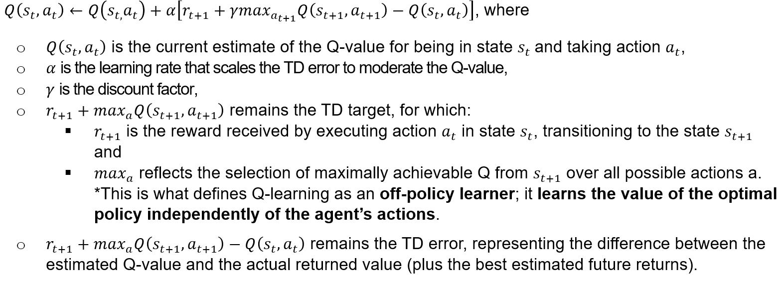
Altogether, the update rule adjusts the Q-value [Q(s_t, a_t)] towards the sum of the reward received for the current action r_(t+1) and the discounted maximum future reward, which is equivalent to incrementally adjusting its estimate towards what it computes as the optimal returns. In this way, the Q-update rule can allow the agent to learn the optimal policy by continuously refining the estimated expected rewards for each action taken in each state.
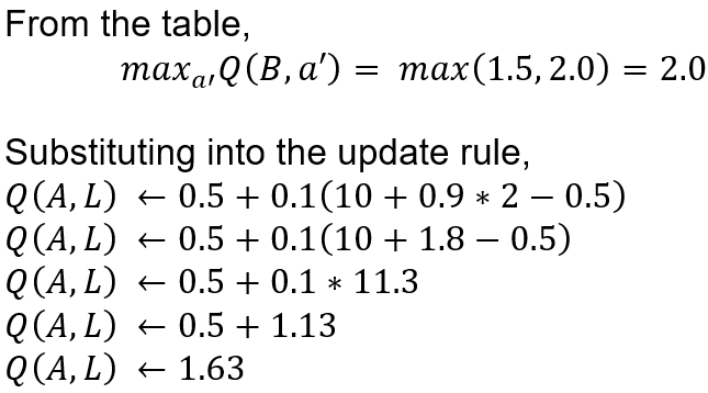
Applying this to the task at hand, we can update Q(A, L) using this formula:

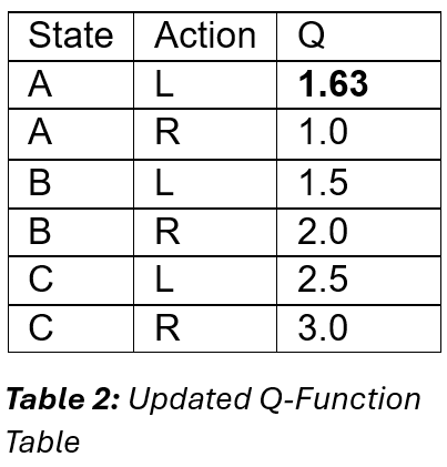
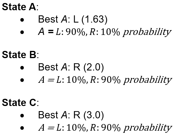
Next, we construct a new policy based on the Updated Q-Function table (Table 2, above) using the ϵ-greedy policy improvement strategy (assuming ϵ = 0.1). To do this, we select the greedy action (i.e., the action that will yield the highest Q-value) with probability 1 – ϵ (0.9) and any other action with probability ϵ (0.1), resulting in a 90% chance of choosing the greedy action and a 10% chance to choose any other action in the state.
The final representation of the ϵ-greedy policy for each state would be:

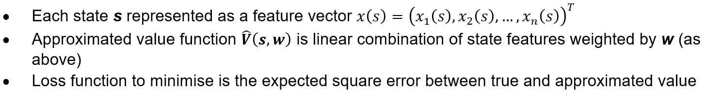
Stochastic Gradient Descent (SGD) Example Using Value Functions
Next, we will explore value functions using the ubiquitous SGD algorithm as an example. The goal will be to design a stochastic gradient descent (SGD) algorithm that trains a weight vector (w) to minimize the mean squared error (MSE) between the true value function (v_pi(s)) and the approximated value function V_hat(s,w) for a given policy pi, where the model is expressed as a weighted linear combination of state features (commonly seen in neural networks).
In using SGD, we are seeking a vector weight w that minimises L(w). To achieve this, we need the gradient of L with respect to w, which requires us to differentiate the loss function (gradient calculation), then we update w (update rule). The expectation can be approximated empirically by sampling states according to policy pi (Kleijn, 2024).
Gradient Calculation:

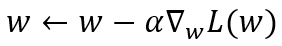
Update Rule:
Given a learning rate α,
This translates to the practical* update rule:
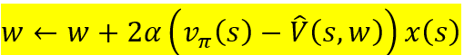
*Note: Does not include backpropagation, as in neural networks.
This is because, unlike NN’s, this is a direct calculation and application of gradients to update the weights, without layered backwards flow of errors that seen in backpropagation.
Pseudocode:
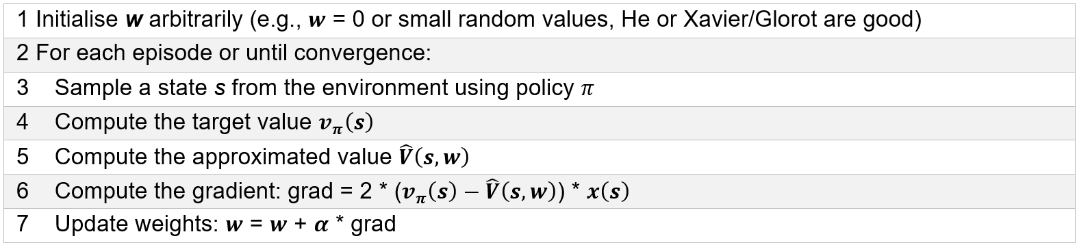
In this way, SGD can be used to iteratively adjust w in the direction that most reduces the discrepancy between the predicted values and the true values under policy pi. By sampling states according to pi, the gradient estimate is aligned with the distribution of states encountered under the actual policy.
References
Amine, A. (2020). Q-Learning Algorithm: From Explanation to Implementation. Medium. https://towardsdatascience.com/q-learning-algorithm-from-explanation-to-implementation-cdbeda2ea187
Chen, A. (2024). AIML431: Dynamic Programming Lecture Notes. Victoria University of Wellington. https://ecs.wgtn.ac.nz/foswiki/pub/Courses/AIML431_2024T2/LectureSchedule/dp.pdf
Kleijn, B. (2024). Basic Deep Learning Regressor & Gradient Descent and Context: AIML425 [Lecture 3 & 4 Notes]. Master of Artificial Intelligence Year One, Victoria University of Wellington. https://ecs.wgtn.ac.nz/foswiki/pub/Courses/AIML425_2024T2/LectureSchedule/DLintro.pdf
