
Background
Markov Decision Processes were formally introduced in the 1950s, with foundational work by Richard Bellman, who developed the concept of dynamic programming and the Bellman equation (discussed later) in 1957. These concepts built on earlier work in stochastic processes and Markov chains by Andrey Markov in the early 20th century. Bellman’s formulation established MDPs as a core mathematical model for sequential decision-making.
Markov Decision Processes (MDPs) remain highly relevant today as the foundational framework for sequential decision-making under uncertainty. They underpin modern reinforcement learning algorithms used in robotics, game-playing agents (e.g. AlphaGo), recommendation systems, and autonomous vehicles. MDPs provide the mathematical structure for modelling environments where outcomes are both probabilistic and dependent on current actions.
One of the best (free) resources on Reinforcement Learning can be found: here.
Defining a Markov Decision Process (MDP)
A Markov Decision Process (MDP) model defining the Shortest Path Problem (SSP) would have a state space, an action space, transition probabilities, rewards, a discount factor, and a goal of determining the optimal policy pi* that maximises the agent’s total expected reward (and consequently, the shortest possible path from node s to node q). To model an SSP we make several assumptions:
- The environment is static;
- Transitions between states are deterministic, i.e., selecting a in s always moves the agent to s’ without randomness);
- Edge weights (costs) c(u,v) are static and known;
- Rewards are static and known; and
- The agent has complete observability (O_t, below), i.e., the model adheres to the basis of an MDP:

The state space {S} = {s_0, s_1, …, s_n, q} consists of all nodes in graph V for the undirected graph G = (V, E). Each state [s belongs to S] corresponds to a node in the graph. The initial state [s_nought] is the starting node and the target state is terminal node q.
For each state s, the action space A(s) includes moving to any adjacent node v where there exists an edge (s, v) in E. Actions are defined by the graph’s adjacency list, which reflects the possible transitions from one node to its neighbors.
The transitions are deterministic. If action a is performed in state s to move the agent to adjacent node v, then the transition probability P(s, a, s’) = 1 for s’ = v and 0 for all other states (s’ does not equal v).
The immediate reward R(s, a, s’) for transitioning from state s to state s’ following action a is the non-negative weight of the edge. We can either swap the maximization for minimization, or more simply, we can define the cost following action a as -c(s, s’). Because all costs are positive, the negative sign ensures that maximising the cummulative reward is equivalent to minimising the total path cost.
The discount factor gamma for future rewards is set to 1 (far-sighted evaluation) because the objective is to minimise the total cost from the start node to the target node without devaluing future path costs. A deterministic optimal policy always exists for an MDP. Optimal policy pi* will provide the direction to move from any node s to the target node q via the shortest path. This policy can be found using dynamic (iterative) programming for value iteration or policy iteration, employing the Bellman Optimality equation:

Once provided a policy pi for our MDP, in the case of iterative policy evaluation, we can use an iterative application of the Bellman expectation backup (synchronous) to calculate the updated value for every non-terminal state. To use dynamic programming to solve the SSP (MDP), we would need to consider two subproblems: prediction, to determine the value function v_pi under the current policy, and control, to determine the optimal value function and policy for MDP: < S, A, P, R, gamma >.
The goal would be to iterate on the value function using a greedy policy (for now, defined as a monotonic, deterministic policy that forcibly follows the best action with respect to the updated value function), running episodes (i.e., iterating) until the process inevitably converges on the optimal value function and policy (see Figure 1, below). Or, mathematically, given a policy pi:

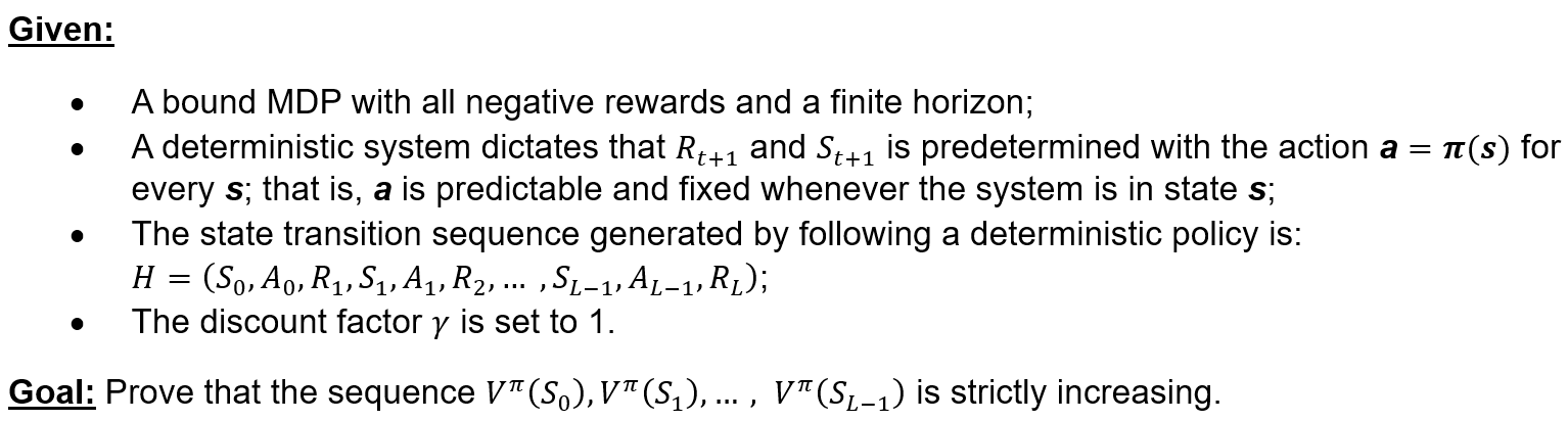
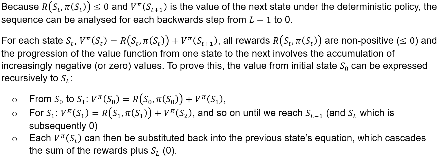
Theoretical Proof: Negative Reward MDP
We will now look at negative reward MDPs using the given example:


References
Amine, A. (2020). Q-Learning Algorithm: From Explanation to Implementation. Medium. https://towardsdatascience.com/q-learning-algorithm-from-explanation-to-implementation-cdbeda2ea187
Chen, A. (2024). AIML431: Dynamic Programming Lecture Notes. Victoria University of Wellington. https://ecs.wgtn.ac.nz/foswiki/pub/Courses/AIML431_2024T2/LectureSchedule/dp.pdf
