[LONG READ | ACADEMIC-STYLE]

1. Background
1.1 Background
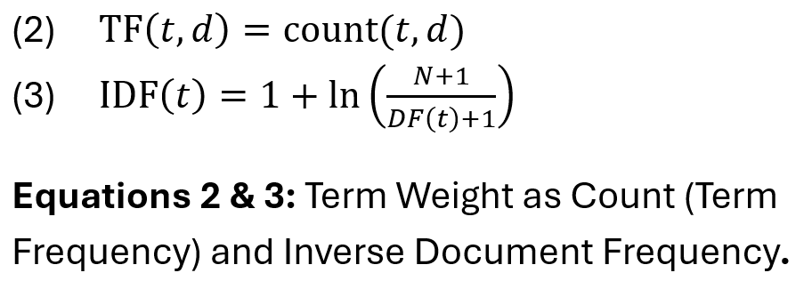
In natural language processing, text must be transformed into numerical representations before it can be consumed by a model. One classical representation is the bag-of-words (BoW) model, in which documents are encoded as vectors of term frequencies, which discard word order but retain counts of each term. However, term frequencies (TF) vary depending on context, topic, domain, style, and so on. This nonstationarity implies that the frequencies of words we observe are averages over contexts. As Piantadosi (2014) formalizes, the probability of uttering a word w is given by:

This equation shows that observed word usage reflects a mixture over hidden contexts, motivating the need for weighted representations like TF×IDF, Term Frequency-Inverse Document Frequency, which account for both local term relevance and global rarity across documents:
Word frequency distributions in natural language often follow a Zipfian or near-Zipfian distribution, where the frequency () of a word is inversely proportional to its rank (
) in the sorted frequency list. The classical form of Zimpf’s Law in equation four characterises term frequencies in terms of their relative proportions to reflect how observed frequencies vary with corpus size (Zipf, 1936, 1949). In practice, “the most frequent word
has a frequency proportional to 1, the second most frequent word
has a frequency proportional to
, the third most frequent word has a frequency proportional to
, and so forth,” i.e., (Piantadosi, 2014):

Zipf’s Law describes a power-law decay in rank frequency (i.e., as rank increases, frequency
decreases polynomially), or equivalently:

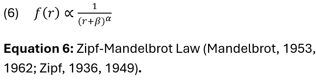
This implies that a small subset of words occurs extremely frequently, while the vast majority of words are rare. However, power-laws decay slowly and tend to have long tails, which often causes the original formulation to overestimate the frequency of rare low-ranked words. To address this limitation, Piantadosi highlights the “current incarnation” of the Zipfian (i.e., near-Zipfian) expression, the Zipf-Mandelbrot law, a generalisation that introduces parameter shift to create a more accurate empirical fit (Piantadosi, 2014).
1.2 Text Prediction and Model Evaluation
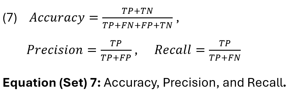
We evaluate the performance of a classical predictive classifier trained on TF representations using a combination of foundational statistics: confusion matrices, accuracy, precision, recall, Fscore (or F1 score), and log loss. A confusion matrix is a tabular representation of a classifier’s performance that records the number of correct and incorrect predictions for each class, providing a granular view of inter-class errors (Fawcett, 2006). From this, key evaluation metrics can be derived: Accuracy measures the overall proportion of all correct predictions but can be misleading in imbalanced settings. Precision class agreement of the data labels with the positive labels given by the classifier, while recall measures the effectiveness of a classifier to identify positive labels (Sokolova & Lapalme, 2009).
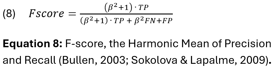
The F-score is the harmonic mean of precision and recall, offering a balanced metric when both false positives and false negatives are relevant (Bullen, 2003). In another way of understanding it, the F-score communicates the relations between data’s positive labels and those given by a classifier (Sokolova & Lapalme, 2009):
Next, we remind ourselves of the theoretical quantities that allow the log loss to evaluate a classifier’s probabilistic confidence by penalising incorrect predictions with high certainty, thus making it a sensitive measure of model calibration. Equation 9 shows that a likelihood is a function to measure how well a model explains observed data (Knott, 2025). In the Bayesian framework, this relationship is formalised via Baye’s Theorem (Equation 10). Here, the likelihood function L(theta) can be represented as P(theta | data), the probability of model parameters theta, given observed data. Despite the likelihood’s formal definition [from probability theory] as a conditional probability of the data given the parameters, it can be reinterpreted as a function (theta) , with the observed data held fixed. This distinction allows it to serve as the central quantity in maximum likelihood estimation (MLE), where likelihood is maximised with respect to theta, and in Bayesian inference, where it shapes the posterior distribution (Kleijn, 2024). Mathematically, this is expressed as:

As Knott 2025 states: “Where all observed corpus events are assumed to be independent, a parameterisable model L(theta) predicts the total probability of all occurrences and iteratively updates its parameters to make this probability as high as possible” (Knott, 2025). This statement describes the statistical inference method for MLE, where we aim to assess the plausibility of model parameters theta given observed data.
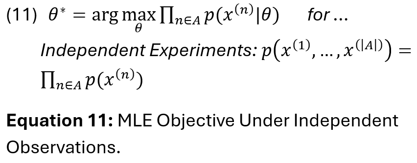
However, because multiplying many small probabilities leads to numerical instability and is difficult to optimise, we instead take the log of the likelihood, turning products into sums to simplify optimisation. This is referred to as the maximum log likelihood (ML) method. It is ubiquitous and does not interfere with the selection of optimal theta (Kleijn, 2024).

In supervised classification, we want to measure how well our model’s predicted probabilities align with the true labels. For this, we can also use the log loss (i.e., cross entropy loss). Unlike accuracy, which simply checks whether the predicted class label is correct, log loss penalises incorrect predictions more harshly when the model is confident, but wrong. The log loss is defined as:
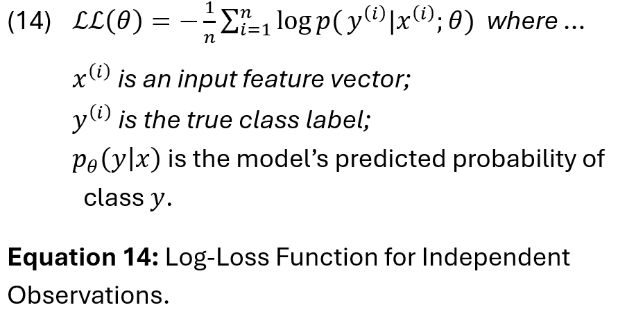
Equation 14 simply expresses the negative average log-likelihood per sample. Moreover, as rigorously established in many standard references on probabilistic modelling and machine learning, minimising the log loss is equivalent to maximising the log-likelihood because minimising the negative of a function is equivalent to maximising the function itself (Murphy, 2012).
1.3 Data Preprocessing
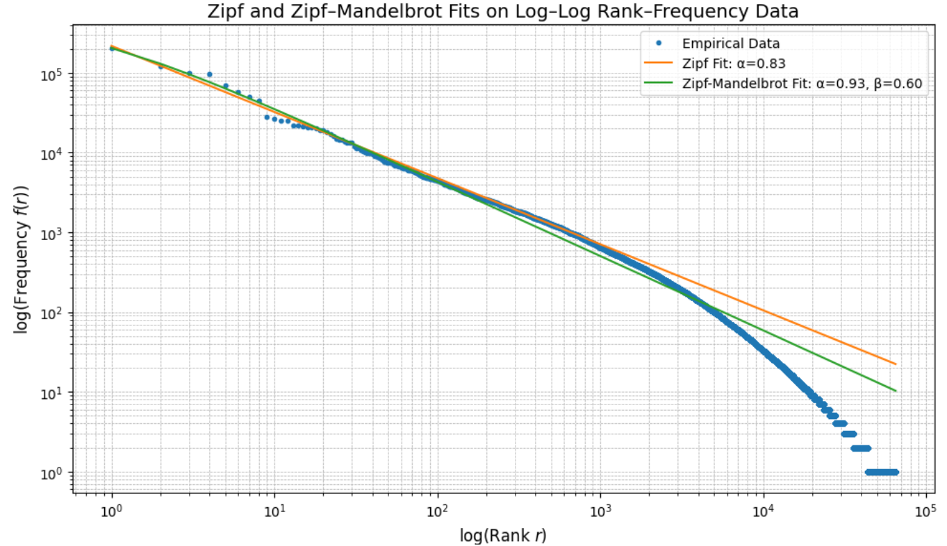
Before modelling a text classifier built on TF representations, we first verified that the training corpus conformed to a Zipfian distribution, such that we might validate the data’s quality and select an appropriate vocabulary size for training. The results of this fitting (Figure 1) indicated that the Zipf-Mandelbrot model had a slightly stronger fit to the empirical distribution than the Zipf model, which slightly underestimated the frequency of common words and overestimated the frequency of rare words:


In the Zipf-Mandelbrot model, the beta-shift reduced the overemphasis of the top 1-2 words and alpha balanced the decay rate more precisely across the rank range:
This suggests that the that the frequency structure of the training corpus is more accurately captured by a near-Zipfian distribution, with 99.1% of the variance explained by the Zipf-Mandelbrot model. Moreover, to quantify the impact of this distribution on term coverage, we performed a Zipfian analysis of our training corpus by plotting the cumulative distribution of term frequencies sorted by descending rank. This allowed us to identify a lexical threshold for the minimum number of distinct terms required to cover a specified proportion of the total token mass (Figure 2). For this particular training corpus, we found that the top 12,382 most frequent terms account for 95% of all term occurrences. Figure 1: Cumulative distribution of term frequencies sorted by descending rank. Figure 2: Zipf and Zipf-Mandelbrot Fit on Log-Log Rank-Frequency Data.
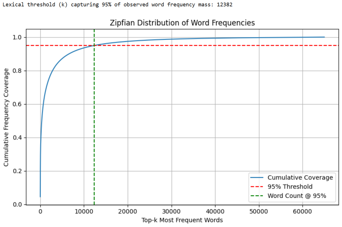

This result indicates that although the raw vocabulary may contain over 65,000 unique terms, the majority of word frequency mass was concentrated in a much smaller subset, as expected. In this way, we were able to limit the vocabulary size to the top 13,000 ranks to reduce model complexity and memory footprint while preserving the most useful signal for classification based on TF representations.
2. TF Classifier
2.1 Model Summary (TF Classifier)
Model one trained a Multinomial Naïve Bayes classifier using only TF representations:
# --------------------------------------------
# TF-IDF Multinominal Naive Bayes Text Classifier:
#    Sklearn CountVectorizer / NB:
#        https://scikit-learn.org/stable/modules/generated/sklearn.feature_extraction.text.CountVectorizer.html
#        https://scikit-learn.org/stable/modules/generated/sklearn.naive_bayes.MultinomialNB.html
#    Max features chosen in preprocessing: 13,000
# --------------------------------------------

import pandas as pd
import numpy as np
from sklearn.feature_extraction.text import CountVectorizer
from sklearn.naive_bayes import MultinomialNB
from sklearn import metrics
from sklearn.metrics import ConfusionMatrixDisplay
from sklearn.metrics import classification_report
from sklearn.metrics import log_loss

# Load data ----------------------
trainDF = pd.read_csv("train.csv")
testDF = pd.read_csv("test.csv")

# Combine 'Title' + 'Description' ----------------------
trainDF['text'] = trainDF['Title'].astype(str) + ' ' + trainDF['Description'].astype(str)
testDF['text'] = testDF['Title'].astype(str) + ' ' + testDF['Description'].astype(str)

# Vectorise (TF only, limit vocab size) ----------------------
vectorizer = CountVectorizer(max_features=13000)
X_train = vectorizer.fit_transform(trainDF['text'])  # sparse
X_test = vectorizer.transform(testDF['text'])

# Class labels
y_train = trainDF['Class Index']
y_test = testDF['Class Index']

# MultinomialNB ----------------------
clf = MultinomialNB()
clf.fit(X_train, y_train)

# Predict and report accuracy ----------------------
train_acc = clf.score(X_train, y_train)
test_acc = clf.score(X_test, y_test)

print(f"Train Accuracy: {train_acc:.6f}")
print(f"Test Accuracy:  {test_acc:.6f}")

# Best practice:
#    Add confusion matrix, precision, recall, F1 score ----------------------
ConfusionMatrixDisplay.from_estimator(clf, X_test, y_test, xticks_rotation=45)
plt.title("Confusion Matrix (Test Set)")
plt.tight_layout()
plt.show()

print(classification_report(y_test, clf.predict(X_test)))

# LL/NLL ----------------------
y_test_proba = clf.predict_proba(X_test)
test_log_loss = log_loss(y_test, y_test_proba, labels=clf.classes_)
print(f"Test Log Loss: {test_log_loss:.4f}")

# Top predictive words per class ----------------------
feature_names = np.array(vectorizer.get_feature_names_out())
for i, class_label in enumerate(clf.classes_):
    top10 = np.argsort(clf.feature_log_prob_[i])[-10:]
    print(f"\nTop words for class {class_label}:")
    print(", ".join(feature_names[top10]))

M1 = {
    "name": "Model 1 - NB on TF Representations",
    "train_acc": train_accs[-1],
    "test_acc": test_accs[-1],
    "test_log_loss": test_log_loss,
    "classification_report": classification_report(y_true, preds, output_dict=True),
    "confusion_matrix": confusion_matrix(y_true, preds)
}
2.2 Model Results (TF Classifier)
The NB classifier trained on TF representations achieved strong overall performance, with a training accuracy of 90.67% and a test accuracy of 89.64%. This relatively small performance gap suggests that the model generalised well to unseen data:

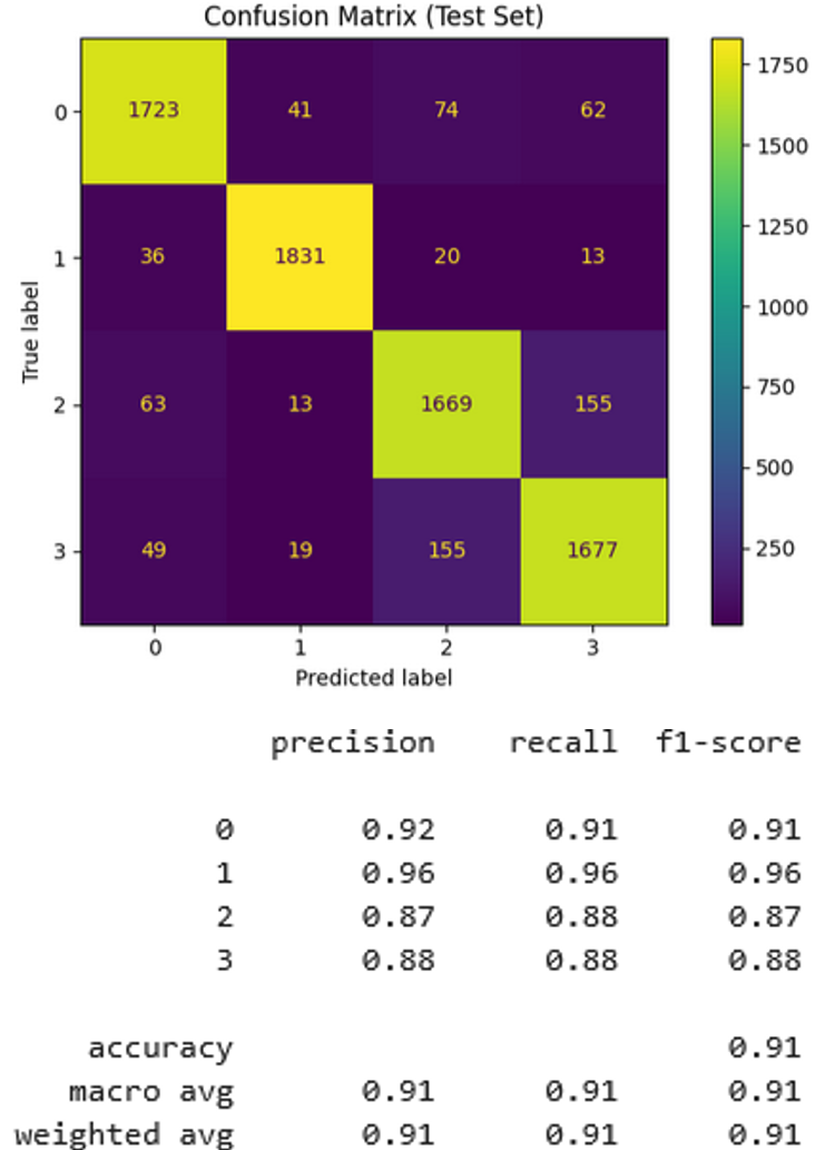
The confusion matrix (Figure 3) and classification report found that class label two had the highest precision and recall at 0.95 and 0.98, indicating that the model had a strong signal for this class. Class three exhibited the most misclassifications at a slightly lower precision and recall of 0.88 and 0.83, suggesting possible semantic overlap or vocabulary similarity between classes three and four. The macro-averaged F1 score is 0.90, indicating balanced performance across classes despite minor inter-class confusion. The log loss of the model was approximately 1.1239. In the context of a four class problem, the theoretical log loss of random assignment (i.e., uniform probability) is:
This means that our model performs better than randomly guessing class labels. Combining all of our results, we can conclude that model one is often right, but not always confident when right, and occasionally confident when wrong.
3. TF-IDF Classifier
3.1 Model Summary (TF-IDF Classifier)
Model two trained a Multinomial Naïve Bayes classifier using TF-IDF representations:
import pandas as pd
import numpy as np
import matplotlib.pyplot as plt
from sklearn.feature_extraction.text import TfidfVectorizer
from sklearn.naive_bayes import MultinomialNB
from sklearn import metrics
from sklearn.metrics import ConfusionMatrixDisplay, classification_report, log_loss

# Load data ----------------------
trainDF = pd.read_csv("train.csv")
testDF = pd.read_csv("test.csv")

# Combine 'Title' + 'Description' ----------------------
trainDF['text'] = trainDF['Title'].astype(str) + ' ' + trainDF['Description'].astype(str)
testDF['text'] = testDF['Title'].astype(str) + ' ' + testDF['Description'].astype(str)

# TF-IDF Vectorisation ----------------------
vectorizer = TfidfVectorizer(max_features=13000)
X_train = vectorizer.fit_transform(trainDF['text'])
X_test = vectorizer.transform(testDF['text'])

# Class labels ----------------------
y_train = trainDF['Class Index']
y_test = testDF['Class Index']

# Multinomial Naïve Bayes classifier ----------------------
clf = MultinomialNB()
clf.fit(X_train, y_train)

# Evaluation Metrics ----------------------
train_acc = clf.score(X_train, y_train)
test_acc = clf.score(X_test, y_test)
print(f"Train Accuracy: {train_acc:.6f}")
print(f"Test Accuracy:  {test_acc:.6f}")


ConfusionMatrixDisplay.from_estimator(clf, X_test, y_test, xticks_rotation=45)
plt.title("Confusion Matrix (Test Set)")
plt.tight_layout()
plt.show()


print(classification_report(y_test, clf.predict(X_test)))

# LL/NLL ----------------------
y_test_proba = clf.predict_proba(X_test)
test_log_loss = log_loss(y_test, y_test_proba, labels=clf.classes_)
print(f"Test Log Loss: {test_log_loss:.4f}")

# Top predictive words per class ----------------------
feature_names = np.array(vectorizer.get_feature_names_out())
for i, class_label in enumerate(clf.classes_):
    top10 = np.argsort(clf.feature_log_prob_[i])[-10:]
    print(f"\nTop words for class {class_label}:")
    print(", ".join(feature_names[top10]))


M2 = {
    "name": "Model 2 - NB on TF-IDF Representations",
    "train_acc": train_accs[-1],
    "test_acc": test_accs[-1],
    "test_log_loss": test_log_loss,
    "classification_report": classification_report(y_true, preds, output_dict=True),
    "confusion_matrix": confusion_matrix(y_true, preds)
}
3.2 Model Results (TF-IDF Classifier)
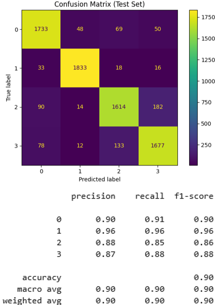
The NB classifier trained on TF-IDF representations achieved slightly better performance than model one. The overall training accuracy was 90.90% and the test accuracy was 89.71%, again indicating that the model two generalised equally well to unseen data as model one.

The confusion matrix (Figure 4) and classification report found that class label two remained the highest in precision and recall (0.95 and 0.98). Class three exhibited the most misclassifications at a slightly lower precision and recall of 0.87 and 0.84, suggesting that model two very marginally improved classification for class 3, its weakest class, as also indicated by a significant decrease in the test log loss at approximately 0.318. The macro-averaged F1 score remained the same (0.90), indicating balanced performance across classes despite some inter-class confusions. Combining this result with our confusion matrix, classification report, and high rate of correct top-class predictions (accuracy), we can conclude that the performance differences between models one and two are negligible.
4. Convolutional Neural Network (CNN) Classifier (1 of 3)
4.1 Model Summary (CNN Classifier, Bespoke Embeddings)
Model three was a Convolutional Neural Network (CNN)-based text classifier implemented in JAX/Flax, using bespoke embeddings.
The model began with a trainable embedding layer that mapped each of the 70 input tokens to a 128-dimensional vector space. The embedded sequence was then processed by a 1D convolutional layer with 128 filters and a kernel size of 5, followed by a ReLU activation. A global average pooling layer reduced the temporal dimension, and the resulting vector was passed through a dense (fully connected) layer that output logits for the 4 target classes. Logits represent unnormalised scores used to calculate the final classification probabilities via a softmax function. Here, softmax activation was applied implicitly through the use of a cross-entropy loss function to suit the multiclass nature of the problem.
# --------------------------------------------
# CNN-based Text Classifier:
# JAX/Flax
# Bespoke embedding training
# Default parameters from class example
# Kernel size: 5 (from class example)
# Necessary adaptations from class example:
# Softmax ---> for multiclass (cross entropy)
# --------------------------------------------
import jax
import jax.numpy as jnp
import numpy as np
import optax
from flax import linen as nn
from flax.training import train_state
from sklearn.model_selection import train_test_split
from sklearn.preprocessing import LabelEncoder
from sklearn.metrics import accuracy_score, classification_report, confusion_matrix, ConfusionMatrixDisplay, log_loss
from collections import Counter
import matplotlib.pyplot as plt
import pandas as pd
import time
# Data Preprocessing ----------------------
def tokenize(texts, vocab=None, unk_token="<UNK>", pad_token="<PAD>", max_len=70):
tokenized = [t.lower().split() for t in texts]
if vocab is None:
tokens = [tok for doc in tokenized for tok in doc]
counts = Counter(tokens)
vocab = {word: i + 2 for i, (word, _) in enumerate(counts.items())} # 0 reserved for PAD, 1 for UNK
vocab[pad_token] = 0
vocab[unk_token] = 1
sequences = []
for doc in tokenized:
ids = [vocab.get(w, vocab[unk_token]) for w in doc[:max_len]]
padded = ids + [vocab[pad_token]] * (max_len - len(ids))
sequences.append(padded[:max_len])
return jnp.array(sequences), vocab
# CNN Text Classifier ----------------------
class TextCNN(nn.Module):
vocab_size: int
embed_dim: int
num_classes: int
@nn.compact
def __call__(self, x):
emb = nn.Embed(self.vocab_size, self.embed_dim)(x)
emb = emb.transpose((0, 2, 1)) # (batch, embed_dim, seq_len)
conv = nn.Conv(features=128, kernel_size=(5,), strides=(1,), padding="VALID")(emb)
conv = nn.relu(conv)
pooled = jnp.mean(conv, axis=-1) # global average pooling (class example)
out = nn.Dense(self.num_classes)(pooled)
return out
# Training Setup ----------------------
def cross_entropy_loss(logits, labels): # cross entropy loss
one_hot = jax.nn.one_hot(labels, num_classes=logits.shape[-1])
return optax.softmax_cross_entropy(logits=logits, labels=one_hot).mean()
def compute_metrics(logits, labels):
predictions = jnp.argmax(logits, axis=-1)
acc = jnp.mean(predictions == labels)
return acc
def create_train_state(rng, model, learning_rate):
params = model.init(rng, jnp.ones((1, 70), jnp.int32))
tx = optax.adam(learning_rate)
return train_state.TrainState.create(apply_fn=model.apply, params=params, tx=tx)
# Main Training Loop ----------------------
def train_model(trainX, trainY, testX, testY, vocab_size, num_classes, num_epochs=25):
model = TextCNN(vocab_size=vocab_size, embed_dim=128, num_classes=num_classes)
rng = jax.random.PRNGKey(0)
state = create_train_state(rng, model, learning_rate=0.01)
train_accs = []
test_accs = []
for epoch in range(num_epochs):
def loss_fn(params):
logits = model.apply(params, trainX)
return cross_entropy_loss(logits, trainY), logits
grad_fn = jax.value_and_grad(loss_fn, has_aux=True)
(loss, logits), grads = grad_fn(state.params)
state = state.apply_gradients(grads=grads)
train_acc = compute_metrics(logits, trainY)
test_logits = model.apply(state.params, testX)
test_acc = compute_metrics(test_logits, testY)
train_accs.append(float(train_acc))
test_accs.append(float(test_acc))
print(f"Epoch {epoch+1}, Train Acc: {train_acc:.4f}, Test Acc: {test_acc:.4f}")
return state, train_accs, test_accs, model
# Data Loading & Execution ----------------------
start_time = time.time()
train_df = pd.read_csv("train.csv")
test_df = pd.read_csv("test.csv")
train_texts = train_df['Title'].astype(str) + ' ' + train_df['Description'].astype(str)
test_texts = test_df['Title'].astype(str) + ' ' + test_df['Description'].astype(str)
trainX, vocab = tokenize(train_texts.tolist(), max_len=70)
testX, _ = tokenize(test_texts.tolist(), vocab=vocab, max_len=70)
le = LabelEncoder()
trainY = jnp.array(le.fit_transform(train_df['Class Index']))
testY = jnp.array(le.transform(test_df['Class Index']))
state, train_accs, test_accs, model = train_model(trainX, trainY, testX, testY, vocab_size=len(vocab), num_classes=4, num_epochs=25)
end_time = time.time()
print(f"\nTotal training time: {end_time - start_time:.2f} seconds.\n")
# Accuracy Plot (Rolling Average for smoothing) ----------------------
def moving_average(data, window_size=6):
return np.convolve(data, np.ones(window_size)/window_size, mode='valid')
smoothed_train = moving_average(train_accs, window_size=10)
smoothed_test = moving_average(test_accs, window_size=10)
epochs = np.arange(len(smoothed_train)) + 1
plt.plot(epochs, smoothed_train, label='Train Accuracy (smoothed)')
plt.plot(epochs, smoothed_test, label='Test Accuracy (smoothed)')
plt.xlabel('Epoch')
plt.ylabel('Accuracy')
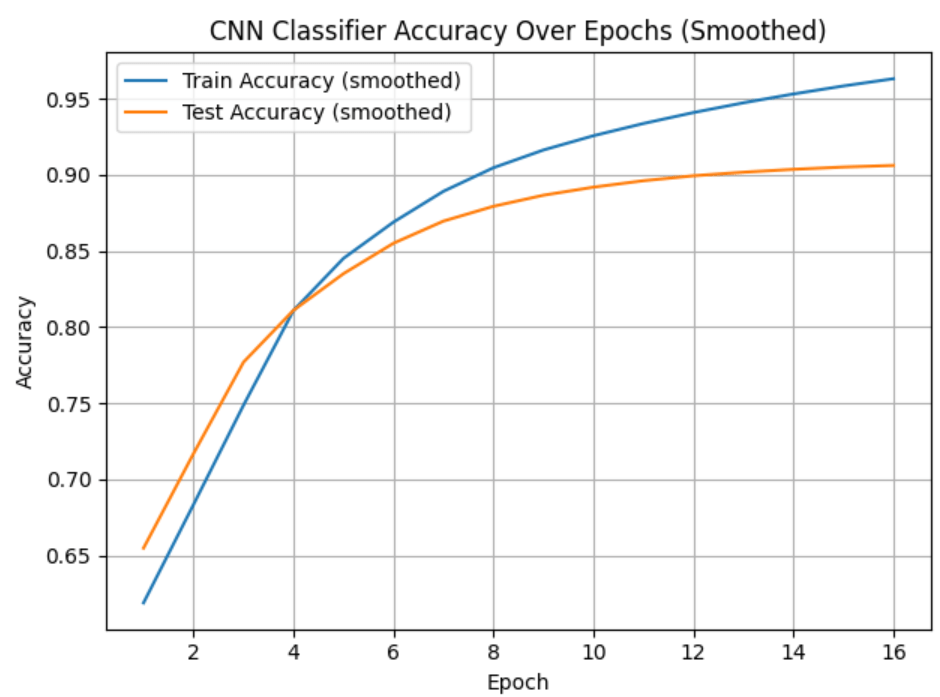
plt.title('CNN Classifier Accuracy Over Epochs (Smoothed)')
plt.legend()
plt.grid(True)
plt.tight_layout()
plt.show()
# Evaluation Metrics ----------------------
final_logits = model.apply(state.params, testX)
preds = np.array(jnp.argmax(final_logits, axis=-1))
y_true = np.array(testY)
print("\nClassification Report:")
print(classification_report(y_true, preds))
probs = jax.nn.softmax(final_logits, axis=-1)
test_log_loss = log_loss(y_true, probs, labels=np.unique(y_true))
print(f"Log Loss: {test_log_loss:.4f}")
print("\nConfusion Matrix:")
ConfusionMatrixDisplay.from_predictions(y_true, preds)
plt.title("Confusion Matrix (Test Set)")
plt.tight_layout()
plt.show()
M3 = {
"name": "Model 3 - CNN with Trainable Embeddings",
"train_acc": train_accs[-1],
"test_acc": test_accs[-1],
"test_log_loss": test_log_loss,
"classification_report": classification_report(y_true, preds, output_dict=True),
"confusion_matrix": confusion_matrix(y_true, preds)
}4.2 Model Results (CNN Classifier, Bespoke Embeddings)
Model three’s performance was comparable to model two. Model three’s overall training and testing accuracy reached 98.05% and 90.79%, respectively. The log loss was a bit higher than the NB/TF-IDF representations, despite some improvements in class 3 and class 4 classifications (Figure 5). Overall, our baseline CNN trained on token embeddings performed similarly to our NB/TF-IDF model, but took approximately 2-3x’s longer to run.
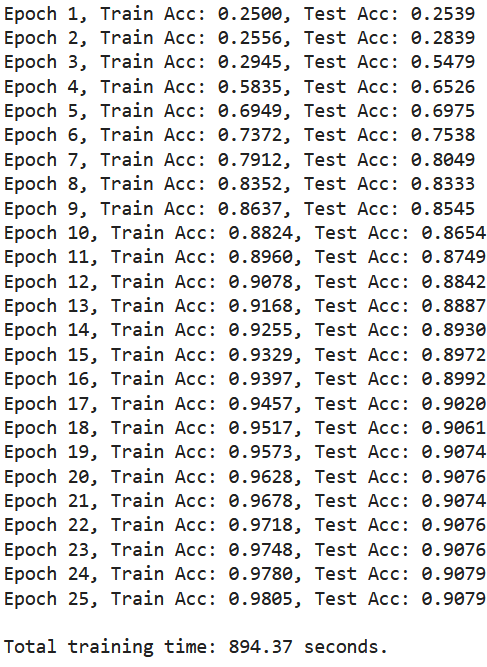
M3 Log Loss: 0.3361
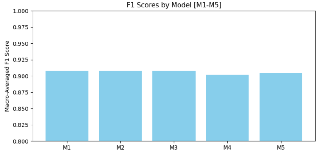
Model three also reported the highest F1-score of 0.91 compared to all other models at 0.90, however this may not represent a statistically significant difference in overall precision.
5. Convolutional Neural Network (CNN) Classifier (2 of 3)
5.1 Model Summary (CNN Classifier, GloVe Embeddings)
Model four was another CNN-based text classifier implemented using JAX/Flax.
It began with a non-trainable embedding layer initialised with 100-dimensional pre-trained GloVe embeddings. Each input sequence was padded/truncated to 53 tokens (adapted to 95th percentile). The embedded input was processed by a 1D convolutional layer with 64 filters and a kernel size of 3, followed by a ReLU activation. A global max pooling layer was used in place of an average pooling layer to reduce the temporal dimension to fixed-size representation. This intermediate output then passed through another dense layer to produce logits for the 4 target classes. We once again applied a softmax distribution implicitly using the multiclass cross-entropy loss function during training.
# --------------------------------------------
# CNN-based Text Classifier:
#    JAX/Flax
#    GloVe Embeddings:
#        https://nlp.stanford.edu/projects/glove/
#    Improved parameters (from step 5)
#
#    Other references:
#        1 - https://flax-linen.readthedocs.io/en/latest/api_reference/flax.linen/module.html
#        2 - https://coderzcolumn.com/tutorials/artificial-intelligence/flax-jax-text-classification-using-glove-embeddings
# --------------------------------------------

import jax
import jax.numpy as jnp
import numpy as np
import optax
from flax import linen as nn
from flax.training import train_state
from sklearn.model_selection import train_test_split
from sklearn.preprocessing import LabelEncoder
from sklearn.metrics import accuracy_score, classification_report, confusion_matrix, ConfusionMatrixDisplay, log_loss
from collections import Counter
import matplotlib.pyplot as plt
import pandas as pd
import time

# Load GloVe Embeddings ----------------------
def load_glove_embeddings(glove_file_path, embedding_dim):
    embeddings_index = {}
    with open(glove_file_path, encoding='utf8') as f:
        for line in f:
            values = line.split()
            word = values[0]
            coefs = np.asarray(values[1:], dtype='float32')
            embeddings_index[word] = coefs
    return embeddings_index

# Data Preprocessing ----------------------
def tokenize(texts, vocab=None, unk_token="<UNK>", pad_token="<PAD>", max_len=53):
    tokenized = [t.lower().split() for t in texts]
    if vocab is None:
        tokens = [tok for doc in tokenized for tok in doc]
        counts = Counter(tokens)
        vocab = {word: i + 2 for i, (word, _) in enumerate(counts.items())}  # 0 reserved for PAD, 1 for UNK
        vocab[pad_token] = 0
        vocab[unk_token] = 1
    sequences = []
    for doc in tokenized:
        ids = [vocab.get(w, vocab[unk_token]) for w in doc[:max_len]]
        padded = ids + [vocab[pad_token]] * (max_len - len(ids))
        sequences.append(padded[:max_len])
    return jnp.array(sequences), vocab

# CNN (Pretrained Embeddings) ----------------------
class TextCNNPretrained(nn.Module):
    embedding_matrix: jnp.ndarray
    num_classes: int

    @nn.compact
    def __call__(self, x):
        emb = nn.Embed(self.embedding_matrix.shape[0], self.embedding_matrix.shape[1], embedding_init=lambda *_: self.embedding_matrix, name="embed", dtype=jnp.float32)(x)
        emb = emb.transpose((0, 2, 1))
        conv = nn.Conv(features=64, kernel_size=(3,), strides=(1,), padding="VALID")(emb)
        conv = nn.relu(conv)
        pooled = jnp.max(conv, axis=-1) # max pooling (preference)
        out = nn.Dense(self.num_classes)(pooled)
        return out

# Training Setup ----------------------
def cross_entropy_loss(logits, labels):
    one_hot = jax.nn.one_hot(labels, num_classes=logits.shape[-1])
    return optax.softmax_cross_entropy(logits=logits, labels=one_hot).mean()

def compute_metrics(logits, labels):
    predictions = jnp.argmax(logits, axis=-1)
    acc = jnp.mean(predictions == labels)
    return acc

def create_train_state(rng, model, learning_rate):
    params = model.init(rng, jnp.ones((1, 53), jnp.int32))
    tx = optax.adam(learning_rate)
    return train_state.TrainState.create(apply_fn=model.apply, params=params, tx=tx)

# Training Loop ----------------------
def train_model(trainX, trainY, testX, testY, embedding_matrix, num_classes, num_epochs=35):
    model = TextCNNPretrained(embedding_matrix=jnp.array(embedding_matrix), num_classes=num_classes)
    rng = jax.random.PRNGKey(0)
    state = create_train_state(rng, model, learning_rate=0.01)

    train_accs = []
    test_accs = []

    for epoch in range(num_epochs):
        def loss_fn(params):
            logits = model.apply(params, trainX)
            return cross_entropy_loss(logits, trainY), logits
        grad_fn = jax.value_and_grad(loss_fn, has_aux=True)
        (loss, logits), grads = grad_fn(state.params)
        state = state.apply_gradients(grads=grads)

        train_acc = compute_metrics(logits, trainY)
        test_logits = model.apply(state.params, testX)
        test_acc = compute_metrics(test_logits, testY)

        train_accs.append(float(train_acc))
        test_accs.append(float(test_acc))
        print(f"Epoch {epoch+1}, Train Acc: {train_acc:.4f}, Test Acc: {test_acc:.4f}")

    return state, train_accs, test_accs, model

# Load Data ----------------------
start_time = time.time()

train_df = pd.read_csv("train.csv")
test_df = pd.read_csv("test.csv")
train_texts = train_df['Title'].astype(str) + ' ' + train_df['Description'].astype(str)
test_texts = test_df['Title'].astype(str) + ' ' + test_df['Description'].astype(str)

trainX, vocab = tokenize(train_texts.tolist(), max_len=53)
testX, _ = tokenize(test_texts.tolist(), vocab=vocab, max_len=53)

embedding_dim = 100
glove_path = "glove.6B.100d.txt"
glove_embeddings = load_glove_embeddings(glove_path, embedding_dim)

embedding_matrix = np.zeros((len(vocab), embedding_dim))
for word, i in vocab.items():
    embedding_vector = glove_embeddings.get(word)
    if embedding_vector is not None:
        embedding_matrix[i] = embedding_vector

le = LabelEncoder()
trainY = jnp.array(le.fit_transform(train_df['Class Index']))
testY = jnp.array(le.transform(test_df['Class Index']))

state, train_accs, test_accs, model = train_model(trainX, trainY, testX, testY, embedding_matrix=embedding_matrix, num_classes=4)

end_time = time.time()
print(f"\nTotal training time: {end_time - start_time:.2f} seconds\n")

# Accuracy Plot ----------------------
def moving_average(data, window_size=6):
    return np.convolve(data, np.ones(window_size)/window_size, mode='valid')

smoothed_train = moving_average(train_accs, window_size=10)
smoothed_test = moving_average(test_accs, window_size=10)

epochs = np.arange(len(smoothed_train)) + 1

plt.plot(epochs, smoothed_train, label='Train Accuracy (smoothed)')
plt.plot(epochs, smoothed_test, label='Test Accuracy (smoothed)')
plt.xlabel('Epoch')
plt.ylabel('Accuracy')
plt.title('CNN Classifier Accuracy Over Epochs (Smoothed)')
plt.legend()
plt.grid(True)
plt.tight_layout()
plt.show()

# Evaluation ----------------------
final_logits = model.apply(state.params, testX)
preds = np.array(jnp.argmax(final_logits, axis=-1))
y_true = np.array(testY)

print("\nClassification Report:")
print(classification_report(y_true, preds))

probs = jax.nn.softmax(final_logits, axis=-1)
test_log_loss = log_loss(y_true, probs, labels=np.unique(y_true))
print(f"Log Loss: {test_log_loss:.4f}")

print("\nConfusion Matrix:")
ConfusionMatrixDisplay.from_predictions(y_true, preds)
plt.title("Confusion Matrix (Test Set)")
plt.tight_layout()
plt.show()

M4 = {
    "name": "Model 4 - CNN with 6B 100d GloVe (Pretrained Embeddings)",
    "train_acc": train_accs[-1],
    "test_acc": test_accs[-1],
    "test_log_loss": test_log_loss,
    "classification_report": classification_report(y_true, preds, output_dict=True),
    "confusion_matrix": confusion_matrix(y_true, preds)
}
5.2 Model Results (CNN Classifier, GLoVe Embeddings)
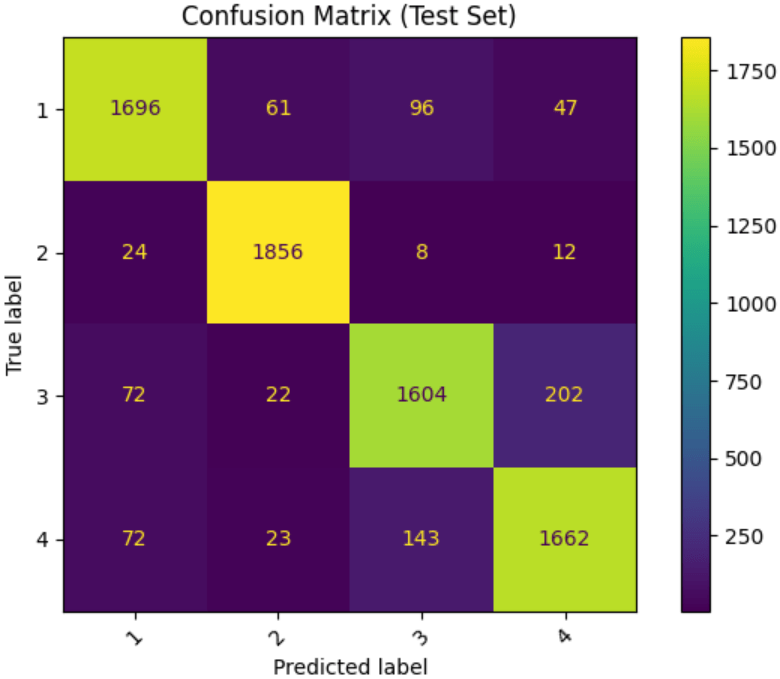
Model four performed significantly better than previous models. It achieved a final training and testing accuracy of 96.92% and 90.22%, respectively.


M4 Log Loss: 0.2884
There remained similar levels of misclassification between classes three and four (Figure 6). However, the log loss was 0.2884, meaning the model had higher confidence in its correct predictions. Further, the model’s run time was halved compared to model three, making it both more accurate and efficient than previous models.
6. Convolutional Neural Network (CNN) Classifier (3 of 3)
6.1 Model Summary (CNN Classifier, Modified)
Model five was another CNN-based text classifier implemented in JAX/Flax.
This model used the same core architecture as model four, but used training, testing, and validation sets, and introduced the Natural Language Tool Kit (NLTK) library for data preprocessing. This model used NLTK tools to enhance data preprocessing by excluding stopwords (e.g., “the”, “is”, “in”) and cleaning stemmed words (e.g., “jumping” -> ”jump”, “loved” -> ”love”, etc.). Here, stemming was applied to each word in the cleaned test after the removal of stopwords.
# --------------------------------------------------
# Lower to 95th-percentile threshold for performance
# --------------------------------------------------

import matplotlib.pyplot as plt
import numpy as np

lengths = [len(text.split()) for text in train_df['Title'] + ' ' + train_df['Description']]
plt.hist(lengths, bins=50)
plt.xlabel("Token Count")
plt.ylabel("Frequency")
plt.title("Distribution of Text Lengths")
plt.show()

# Combine + tokenize
combined_texts = (train_df['Title'] + ' ' + train_df['Description']).astype(str)
lengths = [len(text.lower().split()) for text in combined_texts]

# Compute percentiles
percentiles = [50, 75, 90, 95, 99, 100]
results = np.percentile(lengths, percentiles)

for p, val in zip(percentiles, results):
    print(f"{p}th percentile: {int(val)} tokens")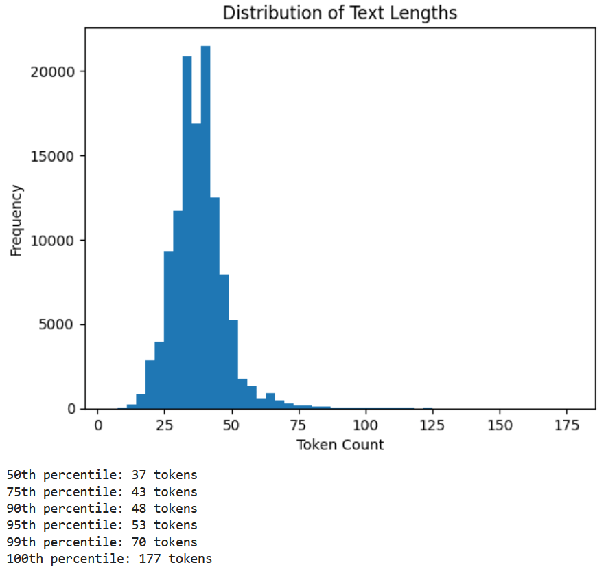
# --------------------------------------------
# CNN-based Text Classifier:
#    JAX/Flax
#    GloVe Embeddings
#    Improved parameters
#    Data Preprocessing
#    Validation Split
#
#    Other references:
#        1 - https://flax-linen.readthedocs.io/en/latest/api_reference/flax.linen/module.html
#        2 - https://www.nltk.org/api/nltk.corpus.html#module-nltk.corpus
#        3 - https://www.nltk.org/api/nltk.stem.html#module-nltk.stem
# --------------------------------------------

import jax
import jax.numpy as jnp
import numpy as np
import optax
from flax import linen as nn
from flax.training import train_state
from sklearn.model_selection import train_test_split
from sklearn.preprocessing import LabelEncoder
from sklearn.metrics import accuracy_score, classification_report, confusion_matrix, ConfusionMatrixDisplay, log_loss
from collections import Counter
import matplotlib.pyplot as plt
import pandas as pd
import time
import re
import nltk
from nltk.corpus import stopwords
from nltk.stem import PorterStemmer
nltk.download('stopwords')

# Load GloVe Embeddings ----------------------
def load_glove_embeddings(glove_file_path, embedding_dim):
    embeddings_index = {}
    with open(glove_file_path, encoding='utf8') as f:
        for line in f:
            values = line.split()
            word = values[0]
            coefs = np.asarray(values[1:], dtype='float32')
            embeddings_index[word] = coefs
    return embeddings_index

# Data Preprocessing ----------------------
def clean_and_tokenize(texts, stop_words, stemmer, rare_threshold=2):
    tokenized_texts = []
    token_freq = Counter()
    for t in texts:
        t = re.sub(r"[^a-zA-Z\s]", "", t.lower())
        tokens = [stemmer.stem(w) for w in t.split() if w not in stop_words]
        tokenized_texts.append(tokens)
        token_freq.update(tokens)
    # Remove rare tokens:
    filtered_texts = [[tok for tok in doc if token_freq[tok] >= rare_threshold] for doc in tokenized_texts]
    return filtered_texts

def tokenize_from_cleaned(tokenized, vocab=None, unk_token="<UNK>", pad_token="<PAD>", max_len=53):
    if vocab is None:
        tokens = [tok for doc in tokenized for tok in doc]
        counts = Counter(tokens)
        vocab = {word: i + 2 for i, (word, _) in enumerate(counts.items())}
        vocab[pad_token] = 0
        vocab[unk_token] = 1
    sequences = []
    for doc in tokenized:
        ids = [vocab.get(w, vocab[unk_token]) for w in doc[:max_len]]
        padded = ids + [vocab[pad_token]] * (max_len - len(ids))
        sequences.append(padded[:max_len])
    return jnp.array(sequences), vocab

# CNN with Pretrained Embeddings ----------------------
class TextCNNPretrained(nn.Module):
    embedding_matrix: jnp.ndarray
    num_classes: int

    @nn.compact
    def __call__(self, x):
        emb = nn.Embed(self.embedding_matrix.shape[0], self.embedding_matrix.shape[1], embedding_init=lambda *_: self.embedding_matrix, name="embed", dtype=jnp.float32)(x)
        emb = emb.transpose((0, 2, 1))
        conv = nn.Conv(features=64, kernel_size=(3,), strides=(1,), padding="VALID")(emb)
        conv = nn.relu(conv)
        pooled = jnp.max(conv, axis=-1)
        out = nn.Dense(self.num_classes)(pooled)
        return out

# Training Setup ----------------------
def cross_entropy_loss(logits, labels):
    one_hot = jax.nn.one_hot(labels, num_classes=logits.shape[-1])
    return optax.softmax_cross_entropy(logits=logits, labels=one_hot).mean()

def compute_metrics(logits, labels):
    predictions = jnp.argmax(logits, axis=-1)
    acc = jnp.mean(predictions == labels)
    return acc

def create_train_state(rng, model, learning_rate):
    params = model.init(rng, jnp.ones((1, 53), jnp.int32))
    tx = optax.adam(learning_rate)
    return train_state.TrainState.create(apply_fn=model.apply, params=params, tx=tx)

# Training Loop ----------------------
def train_model(trainX, trainY, validX, validY, embedding_matrix, num_classes, num_epochs=35):
    model = TextCNNPretrained(embedding_matrix=jnp.array(embedding_matrix), num_classes=num_classes)
    rng = jax.random.PRNGKey(0)
    state = create_train_state(rng, model, learning_rate=0.01)

    train_accs = []
    valid_accs = []

    for epoch in range(num_epochs):
        def loss_fn(params):
            logits = model.apply(params, trainX)
            return cross_entropy_loss(logits, trainY), logits
        grad_fn = jax.value_and_grad(loss_fn, has_aux=True)
        (loss, logits), grads = grad_fn(state.params)
        state = state.apply_gradients(grads=grads)

        train_acc = compute_metrics(logits, trainY)
        valid_logits = model.apply(state.params, validX)
        valid_acc = compute_metrics(valid_logits, validY)

        train_accs.append(float(train_acc))
        valid_accs.append(float(valid_acc))
        print(f"Epoch {epoch+1}, Train Acc: {train_acc:.4f}, Validation Acc: {valid_acc:.4f}")

    return state, train_accs, valid_accs, model

# ---------------------- Load and Process Data ----------------------
start_time = time.time()

stop_words = set(stopwords.words('english'))
stemmer = PorterStemmer()

train_df = pd.read_csv("train.csv")
test_df = pd.read_csv("test.csv")

train_texts_raw = train_df['Title'].astype(str) + ' ' + train_df['Description'].astype(str)
test_texts_raw = test_df['Title'].astype(str) + ' ' + test_df['Description'].astype(str)

train_texts_clean = clean_and_tokenize(train_texts_raw.tolist(), stop_words, stemmer)
test_texts_clean = clean_and_tokenize(test_texts_raw.tolist(), stop_words, stemmer)

X_all, vocab = tokenize_from_cleaned(train_texts_clean)
X_test, _ = tokenize_from_cleaned(test_texts_clean, vocab=vocab)

embedding_dim = 100
glove_path = "glove.6B.100d.txt"
glove_embeddings = load_glove_embeddings(glove_path, embedding_dim)

embedding_matrix = np.zeros((len(vocab), embedding_dim))
for word, i in vocab.items():
    embedding_vector = glove_embeddings.get(word)
    if embedding_vector is not None:
        embedding_matrix[i] = embedding_vector

le = LabelEncoder()
y_all = jnp.array(le.fit_transform(train_df['Class Index']))
y_test = jnp.array(le.transform(test_df['Class Index']))

X_train, X_val, y_train, y_val = train_test_split(X_all, y_all, test_size=0.1, random_state=42)

state, train_accs, val_accs, model = train_model(X_train, y_train, X_val, y_val, embedding_matrix=embedding_matrix, num_classes=4)

end_time = time.time()
print(f"\nTotal training time: {end_time - start_time:.2f} seconds")

# ---------------------- Accuracy Plot ----------------------
def moving_average(data, window_size=6):
    return np.convolve(data, np.ones(window_size)/window_size, mode='valid')

smoothed_train = moving_average(train_accs, window_size=10)
smoothed_val = moving_average(val_accs, window_size=10)

epochs = np.arange(len(smoothed_train)) + 1

plt.plot(epochs, smoothed_train, label='Train Accuracy (smoothed)')
plt.plot(epochs, smoothed_val, label='Validation Accuracy (smoothed)')
plt.xlabel('Epoch')
plt.ylabel('Accuracy')
plt.title('CNN Classifier Accuracy Over Epochs (Smoothed)')
plt.legend()
plt.grid(True)
plt.tight_layout()
plt.show()

# ---------------------- Evaluation on Test Set ----------------------
final_logits = model.apply(state.params, X_test)
preds = np.array(jnp.argmax(final_logits, axis=-1))
y_true = np.array(y_test)

print("\nClassification Report:")
print(classification_report(y_true, preds))

probs = jax.nn.softmax(final_logits, axis=-1)
test_log_loss = log_loss(y_true, probs, labels=np.unique(y_true))
print(f"Log Loss: {test_log_loss:.4f}")

print("\nConfusion Matrix:")
ConfusionMatrixDisplay.from_predictions(y_true, preds)
plt.title("Confusion Matrix (Test Set)")
plt.tight_layout()
plt.show()

M5 = {
    "name": "Model 5 - CNN with 6B 100d GloVe and Preprocessing",
    "train_acc": train_accs[-1],
    "val_acc": val_accs[-1],
    "test_log_loss": test_log_loss,
    "classification_report": classification_report(y_true, preds, output_dict=True),
    "confusion_matrix": confusion_matrix(y_true, preds)
}
6.2 Model Results (CNN Classifier, Modified)
Model five achieved a training accuracy of 95.11% and a validation accuracy of 90.97%, which were the highest of all models. The confusion matrix and classification report (Figure 7) show class label 1 maintained the highest precision (0.96) and recall (0.97), while class 2 continued to be the most difficult to classify (recall of 0.85) throughout all practical experiments. The model achieved a log loss of 0.297, which is a relatively negligible loss compared to the previous model.

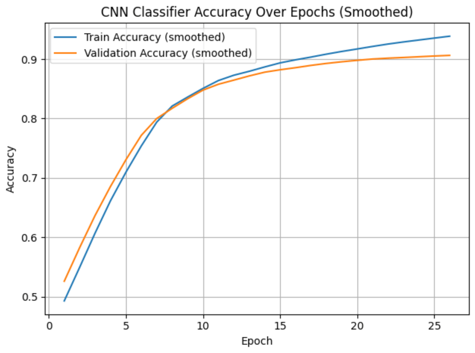
M5 Log Loss: 0.297
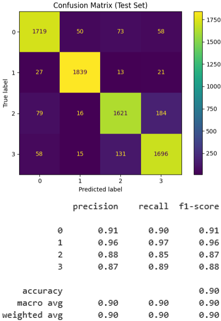
As with most models, the macro-averaged F1 score remained stable at 0.90, reflecting balanced performance across all classes. Collectively, these results suggest that the architectural and preprocessing enhancements slightly affected model calibration and robustness but did not sacrifice overall accuracy or efficiency.
7. Conclusion
Across all models, the CNN classifiers outperformed classical NB approaches in confidence and adaptability, particularly when enhanced with GloVe embeddings and preprocessing techniques. Model five achieved the best overall performance, and successfully balanced accuracy, log loss, and efficiency. These findings underscore the value of data preprocessing, robust embeddings, and careful attention to model design in modern text classification tasks.
ALL Model Comparisons:


References
Bullen, P. S. (2003). The Arithmetic, Geometric and Harmonic Means. In P. S. Bullen (Ed.), Handbook of Means and Their Inequalities (pp. 60–174). Springer Netherlands. https://doi.org/10.1007/978-94-017-0399-4_2
Fawcett, T. (2006). An introduction to ROC analysis. Pattern Recognition Letters, 27(8), 861–874. https://doi.org/https://doi.org/10.1016/j.patrec.2005.10.010
Kleijn, B. (2024). Brief Review Probability Theory and Basic Information Theoric Quantities as Used in Deep Learning: AIML425 [Lecture 1 Notes]. Master of Artificial Intelligence, Victoria University of Wellington, 16–20. https://ecs.wgtn.ac.nz/foswiki/pub/Courses/AIML425_2024T2/LectureSchedule/probability.pdf
Knott, A. (2025). GPT History 1: Neural network language models [AIML428 Lecture Notes]. Master of Artificial Intelligence, Victoria University of Wellington.
Mandelbrot, B. B. (1953). An informational theory of the statistical structure of language. In W. Jackson (Ed.), Communication Theory (pp. 486–502). Butterworths.
Mandelbrot, B. B. (1962). On the theory of word frequencies and on related Markovian models of discourse. In Structure of Language and its Mathematical Aspects (Vol. 12, pp. 190–219). American Mathematical Society.
Murphy, K. P. (2012). Graphical Models and Dynamic Bayesian Networks. In Machine Learning: A Probabilistic Perspective (pp. 247–290). MIT Press.
Piantadosi, S. T. (2014). Zipf’s word frequency law in natural language: A critical review and future directions. Psychonomic Bulletin & Review, 21(5), 1112–1130. https://doi.org/10.3758/s13423-014-0585-6
Sokolova, M., & Lapalme, G. (2009). A systematic analysis of performance measures for classification tasks. Information Processing & Management, 45(4), 427–437. https://doi.org/https://doi.org/10.1016/j.ipm.2009.03.002
Zipf, G. (1936). The Psychobiology of Language. London: Routledge. Zipf, G. (1949). Human Behavior and the Principle of Least Effort. New York: Addison-Wesley.
