[VERY LONG READ | ACADEMIC STYLE]
Section 1: Abstract
In 2025, computer-generated imagery (CGI) and by extension, AI generated content (AIGC), are on track to reach new heights in quality and accessibility with the continued popularisation of deep learning-based video generation frameworks, including large vision and multimodal models like Sora and Vidu [1], [2], [3]. Much of this progress can be attributed to recent advancements in deep learning and generative modeling. Yet, beneath the surface of unprecedented video generation capabilities lie challenges with spatial distortions, spatial control, temporal coherence, and difficulties balancing realism with diversity. Addressing these challenges is crucial not only for advancing the technical robustness of LVMs, but also for realising their full creative potential in practical, real-world applications.
Sectors for entertainment, education, media, and marketing, and specialist subfields like virtual reality and autonomous systems, perhaps stand to benefit the most from LVMs in the immediate future. Of course, uptake is also contingent on unresolved questions about the limits, scalability, and sustainability of industry-grade large generative models. Despite significant breakthroughs across a range of these models in recent years, industry and academia remain leagues away from lofty goals like technical and creative perfection in the technologies available to support end-to-end video synthesis. However, addressing current issues like spatial and temporal coherence requires a deep understanding of the theory, foundations, and contemporary methods observed in state-of-the-art models.
Hence, this literature review aims to, firstly, frame deep learning-based video generation as a modern topic that stems from (and continues to overlap with) the domains of computer vision and computer graphics. Then, we transition from a broad overview of the field to a brief discussion on the theoretical foundations and limitations of Generative Adversarial Networks (GANs), a method that once dominated ‘state-of-the-art’ generative modelling practices, to develop a contextual appreciation for the decline of GANs in favour of diffusion-based methods. Next, we take an in-depth look at the mechanics of diffusion to understand the principles that underpin a significant proportion of contemporary state-of-the-art models. Following this, we outline two crucial classes of challenges in video generation, spatial and temporal coherence, and introduce the role of blocks in mitigating distortions. Afterwards, we provide a high-level overview of Sora, a state-of-the-art model for video generation, to put into perspective cutting-edge approaches that marry all of these complexities to produce incredible results. Finally, we use the findings of this review to compile our closing arguments and propose new directions for future research.
We acknowledge that society, industry, and different domain ideologies have influenced the evolution of video generation and deep learning to varying degrees, and caution that this review is primarily concerned with delivery to a technical audience. Supplementary material is required for a holistic discussion on the ‘evolution of deep learning and its impact on video generation’ [4], [5], [6], [7], [8].
For example, while the scope of this paper is limited to video generation [and closely related] deep learning methods, additional reading is recommended for their discussions on the influence of hardware and computation in enabling such advanced technological capabilities.
The context supplied by these perspectives remains non-exhaustive for a truly holistic discussion, but we hope that they provoke thought about breakthroughs in adjacent areas which, while not covered in this paper, continue to play critical roles in supporting video generation and other deep learning advancements.
Section 3: Transition to Deep Learning
At their core, many early computer vision and graphics approaches were grounded in mathematical modeling and algorithmic ingenuity. They often relied on explicit rules, constraints, or maths to synthesise and manipulate visual data, but had a limited ability to handle complex tasks, generalise well, and accurately simulate photorealism. This ultimately led to gradual shifts away from bespoke methods in favor of machine learning and data-driven techniques.
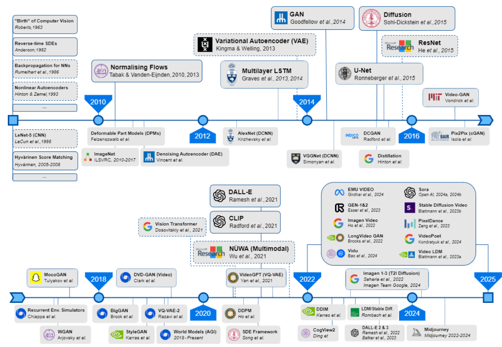
Deep learning sparked significant paradigm shifts for computer vision and image and video generation. Deep learning-based approaches became especially prominent by the mid-2010s when the ‘deep learning revolution’ pervaded the fields of machine learning and data science [14]. From the start of this revolution to date, deep learning models have become increasingly adept at learning visual patterns and representations directly from large datasets. The timeline presented in Figure 1 provides a helpful visual reference of historic to present-day state-of-the-art models.
In 2010, 2013, and 2014, three major breakthroughs reshaped the landscape of image synthesis: normalizing flows [56], [57], Variational Autoencoders (VAEs) [32], and Generative Adversarial Networks (GANs) [58]. Each of these methods introduced foundational advancements in density estimation, latent variable modeling, and adversarial training, respectively.
The next wave of innovation emerged in 2015 with diffusion models [8] and U-Net architectures [59]. Diffusion was presented in the context of generative modelling for the first time, while U-Nets (Ronneberger et al., 2015) introduced a powerful encoder-decoder framework that greatly influenced structured image-to-image translation. Prior to diffusion models and, to some extent alongside them, GANs, Convolutional Neural Networks (CNNs), and their variants (e.g., DCNNs [60] and DCGANs [61], [62]) dominated early deep generative modelling.
CNNs are not covered extensively in this review, but we may briefly acknowledge some of their contributing limitations to the rise of GANs:
In the paper Arguments for the Unsuitability of Convolutional Neural Networks for Non-Local Tasks, Stabinger et al. argue that CNNs struggle with long-range dependency modeling, making them less effective for tasks that require global contextual understanding like image synthesis and scene generation [63].
This is echoed in greater detail in the paper: Theoretical Analysis of Inductive Biases in Deep Convolutional Networks. Here, Wang and Wu describe locality bias as a fundamental limitation of CNNs that restricts their ability to capture relationships beyond a fixed receptive field [64].
At the same time, Residual Networks (ResNets) introduced skip connections, which mitigated vanishing gradients and enabled training to go much deeper in networks [34]. For a time, ResNets were fundamental to high-res image synthesis because they were shown to improve performance and stability in DCNNs and GANs (e.g., BigGAN [65]). When they first emerged, it was also [partly] incorrectly assumed that increasing model depth directly correlated with image quality. Later, research like StyleGAN [66] and StudioGAN [67] proved greater nuance and complexity to this relationship, which supported the idea that model architecture and training methods are at least equally as important as depth. Presently, while some valid investigations into uses for ResNets remain – such as refining VAE encoders and decoders [68], [69] and improving denoising networks in diffusion models [70] – the landscape of deep learning architectures has generally evolved beyond them in favour of transformer-based methods.
When Vaswani et al. published their groundbreaking work on Transformers in 2017 [71], natural language processing (NLP) rapidly flourished, leading to state-of-the-art large language models (LLMs) like ChatGPT, BERT, and more. Roughly three years later, Dosovitskiy et al. brought transformers into the domain of computer vision with their landmark adaptation of the architecture for image recognition at scale, the Vision Transformer (ViT) [72]. Their work demonstrated that the usefulness of parallelisation and attention could extend well beyond text processing (though ‘traditional’ NLP-centred transformers are still commonly found in state-of-the-art multi-modal models, like Sora).
This non-exhaustive overview of advancements highlights the cutting edge of image and video generation. However, a comprehensive technical analysis of all models, methods, and techniques that have shaped the evolution of deep learning for video generation falls beyond the scope of a single literature review.
As such, we transition from this broad overview to a brief discussion on the theoretical foundations and limitations of GANs, the method that once dominated ‘state-of-the-art’ generative modelling practices, to develop contextual appreciation for their decline in favour of diffusion. Following this, we take an in-depth look at the mechanics of diffusion to understand the principles underpinning a significant proportion of contemporary state-of-the-art models. Next, we compare two different bleeding edge diffusion architectures for video generation: stable diffusion with VAEs and diffusion with vision transformers. Finally, we use the findings of this review to compile our closing arguments and propose new directions for research.
Section 4: Theoretical Foundations of GANs
Generative Adversarial Networks (GANs) were first introduced in 2014 by Goodfellow et al. as an adversarial process in which two neural networks compete in a minimax game to improve one another’s performance [58].
At a high level, GANs are networks underpinned by two connected sub-networks, a Generator (G) and a Discriminator (D). The role of the discriminator is to distinguish between real and synthetic images, while the role of the generator is to generate increasingly representative samples of the real distribution. The two networks pass update information through an image (i.e., a high dimensionality vector) and rely on adversarial learning to create mutual updates. This teaches each network to build stronger capabilities for generating and distinguishing detailed information over many iterations. The adversarial process for training a GAN is as follows: First, we randomly initialise the weights. Next, we train discriminator D by fixing G. Then, we fix D and update G to train the generator, inverting real and synthetic labels. In this way, we continue to alternate fixing and updating each sub-network until the system reaches convergence.
The optimal generator and discriminator, G* and D*, can then be computed using binary cross entropy loss to represent real versus fake classifications:

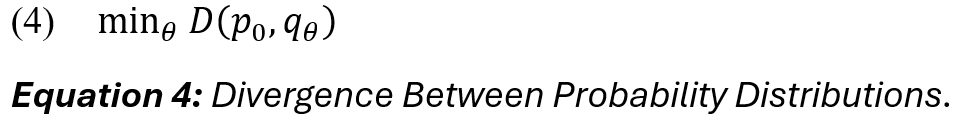
Alternatively, GANs can be understood as divergence minimisation problems. First, we assume that divergence function D takes a pair of probability distributions as input and returns an element from [0, inf] that satisfies D(p, p) = 0 for all probability distributions p. Then, we are given some target distribution p_nought from which we can draw i.i.d. samples and a parametric family of distributions, q_theta (i.e., a neural network) [73]. Our goal is to find the optimal value (theta)* which minimises the divergence: D(p_nought, q_theta):
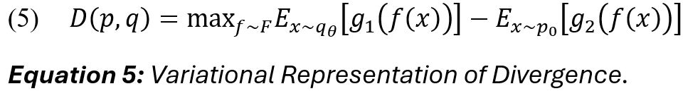
As we know from Goodfellow et al. and earlier works rooted in probability and information theory [74], [75], [76], [77], divergences are commonly expressed in the form (5):
for some function class

and convex functions

As Mescheder points out, (4) and (5) together leads to a minimax optimisation problem of the form:

Thus, the final expression (6) represents the maximum objective value which, in the original formulation of a GAN, is the minimum Jensen-Shannon (JS) divergence of two empirical distributions [58].
Limitations of GANs
Since their inception, GANs have been applied with varying degrees of success to a wide range of generative tasks, including image and video transformation, manipulation, and full image and video synthesis. Some variants, like Deep Convolutional GANs (DCGANs) [61], Wasserstein GANs (WGANs) [78], and Least Squares GANs (LSGANs) [79] achieved state-of-the-art results in image generation at the time of their respective publications. However, the limitations of GANs became more apparent as diffusion models started to outperform them in similar (or identical) generative tasks. This is because, despite demonstrating some of the most impactful innovations in image synthesis in recent history, GANs are also hindered by several inherent limitations – many of which stem from the mathematical instability of the adversarial training framework that underpin all GANs and their variants.
The minimax problem often suffers from non-convergence as the system tries to simultaneously optimise two competing objectives. This causes the gradients to oscillate and leads to numerical instability. One well-known issue is that when P_G and P_data have non-overlapping supports, the Jensen-Shannon (JS) divergence becomes a constant, causing gradients to vanish. As a result, the generator receives little useful signal from the discriminator, making it difficult to learn when the distributions are too far apart.
In 2018, Mescheder et al. provided a detailed account of the numerical challenges associated with training, citing two separate issues with GANs: computationally, no Nash equilibrium exists or it may be degenerate, and algorithmically, we have limited reliable tools for finding Nash equilibria. While the paper proposed an algorithmic method requiring both players to possess negative definite Hessians to improve convergence, it also made it clear that, fundamentally, standard GAN training methods suffer from an inherent instability that prevents reliable convergence in many cases. Mescheder’s analysis of convergence properties for the most common method of training GANs, simultaneous gradient ascent, demonstrated two major failure causes for this system: eigenvalues of the Jacobian of the associated gradient vector field with zero real-part, and eigenvalues with large imaginary part [73].
The theoretical challenges are accompanied by practical consequences, too. When the Jacobian eigenvalues have zero real parts, training slows or stalls, leading to vanishing gradients. When the eigenvalues have large imaginary parts, training oscillates uncontrollably and exacerbates mode collapse. In practice, these instabilities manifest as poor convergence, a collapse of diversity in generated samples, and failed learning dynamics. By extrapolation, it is reasonable to assume that the scope in which GANs remain competitive with diffusion will continue to narrow as diffusion-based approaches further improve in efficiency and scalability.
Despite their pitfalls, GANs have left a lasting impression on cutting-edge methods. For example, distillation methods like Adversarial Diffusion Distillation (ADD) [80] and Fast adversarial diffusion distillation [81] speed up diffusion models by training a student model to replicate the outputs of a performant, slower teacher model in fewer steps using GAN-like adversarial losses. In an adversarial diffusion setup, the GAN criterion introduces a discriminator that pushes the student’s outputs towards a distribution that is indistinguishable from real data by comparing features between the generative outputs of the student and the teacher. The observation of student models successfully trained using a GAN criterion indicates that adversarial losses may still be useful tools for simplifying distribution matching.
Section 5: Theoretical Foundations of Diffusion
Diffusion processes offer a fundamentally different and mathematically stable approach for modelling complex data distributions. In recent years, diffusion methods have gained prominence in generative tasks like image and video synthesis. The core principle behind the approach is to transform data into a simple noise distribution (e.g., Gaussian) using a forward diffusion process, and then reconstruct the original distribution via a learned reverse diffusion process. Different formulations of diffusion may impose various constraints on these transformations and, while most retain the fundamental structure of forward and reverse diffusion processes, some deterministic formulations approximate the dynamics without relying on stochastic diffusion in the reverse process.
In this section, we explore the theoretical foundations of diffusion, describe the derivation of forward and reverse diffusion processes, their variants, and highlight the importance of score-based solving through a discussion justifying components of their mathematical stability. Overall, diffusion approaches address many of the quality and stability challenges observed in other generative models, contributing to their prominence in state-of-the-art image and video synthesis methods.
Derivation of the SDE and Stochastic Diffusion Processes
The first diffusion model used in the context of generative modeling, the Denoising Diffusion Probabilistic Model (DDPM), was derived from the Markov chain and nonequilibrium thermodynamics theory (particle diffusion) [8]. The model is expressed as a forward Markov process (7) (i.e., a system in which the next state depends on all previous states) that gradually replaces a clean signal with Gaussian noise, followed by an approximation of the process’s probabilistic inverse (8) to reconstruct a random variable input using parameter theta [82], [83].

The DDPM motivated the formulation of the Markov chain as an Itô stochastic differential equation (SDE), expressed in general notation as (9). The process reversal can be expressed in terms of the (10) Fokker-Planck equation (FPE), which describes the evolution of the probability density p(x, t) over time via a velocity field (but does not directly describe individual sample paths). Notably, we cannot solve for p(x, t) directly, nor is the FPE immediately useful for reversing a stochastic process in its partial derivative form. The reasons behind this are discussed in greater detail in Section 5.5, Mathematical Stability.
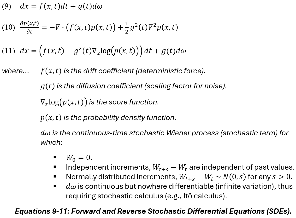
Anderson’s early work provided the first formal derivation of the reverse-time stochastic diffusion process, in which he used the FPE (i.e., Kolmogorov forward equation) to demonstrate the necessity of the drift coefficient during reversal to counteract stochastic spreading in the forward process [46], [84]. However, a non-trivial derivation is required to attain (11), the expression for a reverse-time stochastic differential equation solvable through Hyvärinen score matching [85], [86].
First, we perturb data using SDEs. We refer to tools, such as reverse-time SDEs and Hyvärinen score-based techniques that allow us to model the backward process more efficiently while maintaining probability consistency [46], [85], [87-89]. In this way, instead of solving for p(x, t), we can estimate only its gradient, [nabla_x * log p(x, t)], which is much lower in dimensions and easier to approximate (via a neural network).
One of the most resounding recent contributions to diffusion research has been the unified framework presented by Song et al. “to explore and tune various SDEs for improving score-based generative models,” depicted in Figure 2, below [86].
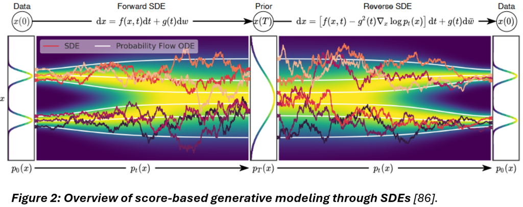
This framework outlines steps and conditions under which to perturb data using SDEs, generate samples by reversing the diffusion process (with what is ultimately another diffusion process given by the reverse-time SDE [46]), and estimate scores for the SDE by training a score-based model on samples with score matching [86].
Next, we generate samples by reversing the SDE using equation (11) and estimate the scores for the SDE.
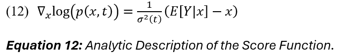
The score function estimates the clean signal based on the difference between the noisy signal x at time t and the clean signal Y. The method used to learn the score function is referred to as score matching. In score matching, the forward process of summing random Gaussian variables is equated to convolving their densities; this is helpful for formulating an analytic description of the score (12):
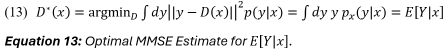
The next step is to define an MMSE estimator D for Y, in which Y is conditional on current data x (13):
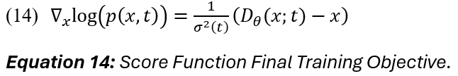
Finally, it is possible to approximate E [ Y | x ] with a D_theta, an all-of-t neural network denoiser [D_theta(x ; t)], by sampling a clean image, selecting a random time t to obtain a controlled noisy signal and gradient step training to reduce the mean squared error between
[D_theta(x ; t)] and clean signal y.
Once the score function [nabla_x * log p(x, t)] is learned via a neural network as a function of x and t, it can be used within the Euler-Maruyama method (2) to solve the backwards SDE (or ODE, discussed further on) [85]. The cumulative process describes the evolution of an X (e.g., an image) and effectively maps one distribution to another. Notably, the reversal is not exact due to the Wiener term (stochasticity) in the forward process, but after many iterations the result still follows the original (intended) distribution.
Limitations of Diffusion
Diffusion models have proven themselves capable of generating some of the highest-quality images and videos, but still possess limitations relating to their iterativeness, inefficiency, and difficulty balancing fidelity with diversity. While there are fewer drawbacks with diffusion than GANs, one significant disadvantage is their computational inefficiency. GANs generate samples in a single forward pass, whereas the iterative denoising steps of diffusion models can be orders of magnitude slower [82], [86].
Techniques like ODE-based approximation [86], [94], [107] and progressive distillation [only briefly mentioned in this review] [97] can be used to reduce the number of inference steps, but often comes at the expense of performance.
Lastly, diffusion processes are presently the most successful generative method for maintaining spatial and temporal coherence amongst high-dimensional correlations inherent in video data. Diffusion-based models inherently address time progression through their temporal component and handle the spatial refinement of frames’ contents and structure over many denoising iterations, but even these methods remain susceptible to spatial and temporal distortions.
Section 6: Maintaining Coherence
Coherence presents some of the hardest classes of challenges in generative image and video modelling. Missing or interrupted coherence can affect the structural integrity and visual continuity of generated outputs. Unlike static image generation, which only requires spatial coherence, high-quality video generation requires both spatial and temporal consistency. In the context of video generation, this dual set of considerations is reflective of models’ need to maintain consistency across frames while capturing complex motion dynamics.
Spatial distortions, such as warping, artefact manifestation, and scaling inconsistencies, disrupt the structural integrity of individual frames, leading to unnatural object appearances or lighting, and misaligned textures. Temporal distortions affect frame-to-frame consistency and, when present, manifest as flickering, jittering, or abrupt changes that break the illusion of continuous motion. To provide variety, this section will explain spatial distortions through a simple illustrative example and discuss temporal distortions from a more traditional theoretical perspective. Additionally, this section will briefly discuss how coherence and lengthier sequences are achieved. Many video generation frameworks adopt a “block-based” approach to control spatial and temporal components, meaning that they process sequences of frames as coherent units. Blocks can be used to control video slices, or segments, that represent a subset of spatial and temporal dependencies. By combining them, we can form longer video sequences that better capture motion patterns and maintain coherence across frames.
Spatial Distortions
Spatial distortions represent the first class of challenges in generative image and video modelling. Spatial distortions can manifest in generated static images or independent frames of videos. Depending on the severity of these distortions, subjects and objects can be perceived as having unnatural lighting or appearance, misaligned textures, and more.
Figure 4 presents a quick illustrative example, highlighting obvious warping and topological distortions in a DALL-E 3 [108](diffusion-based) image generated from the prompt: “An old man waving in the middle of a crowded hotel lobby.”

Qualitative (visual) inspections are often used in conjunction with quantitative measures, particularly in academic settings. Metrics to evaluate generated images are especially useful for detecting more subtle distortions and comparing different models’ performances on generative tasks.
Two of the most common spatial distortions are artefact manifestation, which introduces unintended visual noise or irregularities, and warping, where spatial relationships and object geometries become distorted (i.e., parts of an object appear stretched, compressed, or misaligned, but the fundamental structure is correct, e.g., five fingers, five toes).
Extending the example in Figure 4, a variety of techniques can be employed to detect subtle spatial distortions. For the sake of maintaining a straightforward example that superficially demonstrates the current limitations of ‘state-of-the-art’ (image generation) diffusion models, we can disregard several of the more complex spatial distortions present in the image, such as inconsistencies in perspective, scaling, and texture. Focusing only on artefacts and warping, we refer to Figure 5 for an advanced inspection of the original image.

The first part of our analysis consists of searching the image for checkerboarding, a term commonly used to describe the appearance of grid-like artefacts caused by the interaction between convolutional kernels, stride, and padding during upsampling operations. A convolution is an integral expressing the amount of overlap of a function, [g(.)], as it is shifted over another function,
[f(.)] [109]. The continuous convolution of two functions f(t) and g(t) along grid-like channels, or lower resolution aspects of an image, can be defined as:

Since we are analysing an image (i.e., a discrete matrix), a convolution is instead expressed as a sum:

The transpose convolution, or deconvolution, is used for upsampling and reverses the spatial reduction caused by a standard convolution:

As stated, certain combinations of kernel, padding, and stride can cause pixels in the output to receive more frequent contributions from the kernel. Uneven overlaps lead to periodic patterns in pixel intensities, manifesting checkerboard-like spatial distortions. When we want to inspect an image for such artefacts, we may use Fourier transform (FFT) [110], Structural Similarity Index (SSIM) [111], or a statistical measure that reflects pixel differences. For simplicity, we use the last approach and quantify pixel differences with local entropy.
First, we convert the image to greyscale. Then, we compute the entropy of the vertical and horizontal difference maps (i.e., the horizontal and vertical differences between adjacent pixels). Both difference maps highlight edge-like features in their respective directions. If neighboring pixels differ greatly, there is more uncertainty, indicating higher local entropy. In this example, entropy values are visualised in the form of heat maps seen in Figure 5a.
Entropy, the average information of Z, is expressed as [112]:

Next, we relate this to the distribution as a statistical measure of differences between pixels. Let Z_delta be a random variable representing pixel differences, such that:

Let [p_delta (z_delta)] be the probability distribution of pixel differences across the image. Local entropy based on pixel differences is therefore:
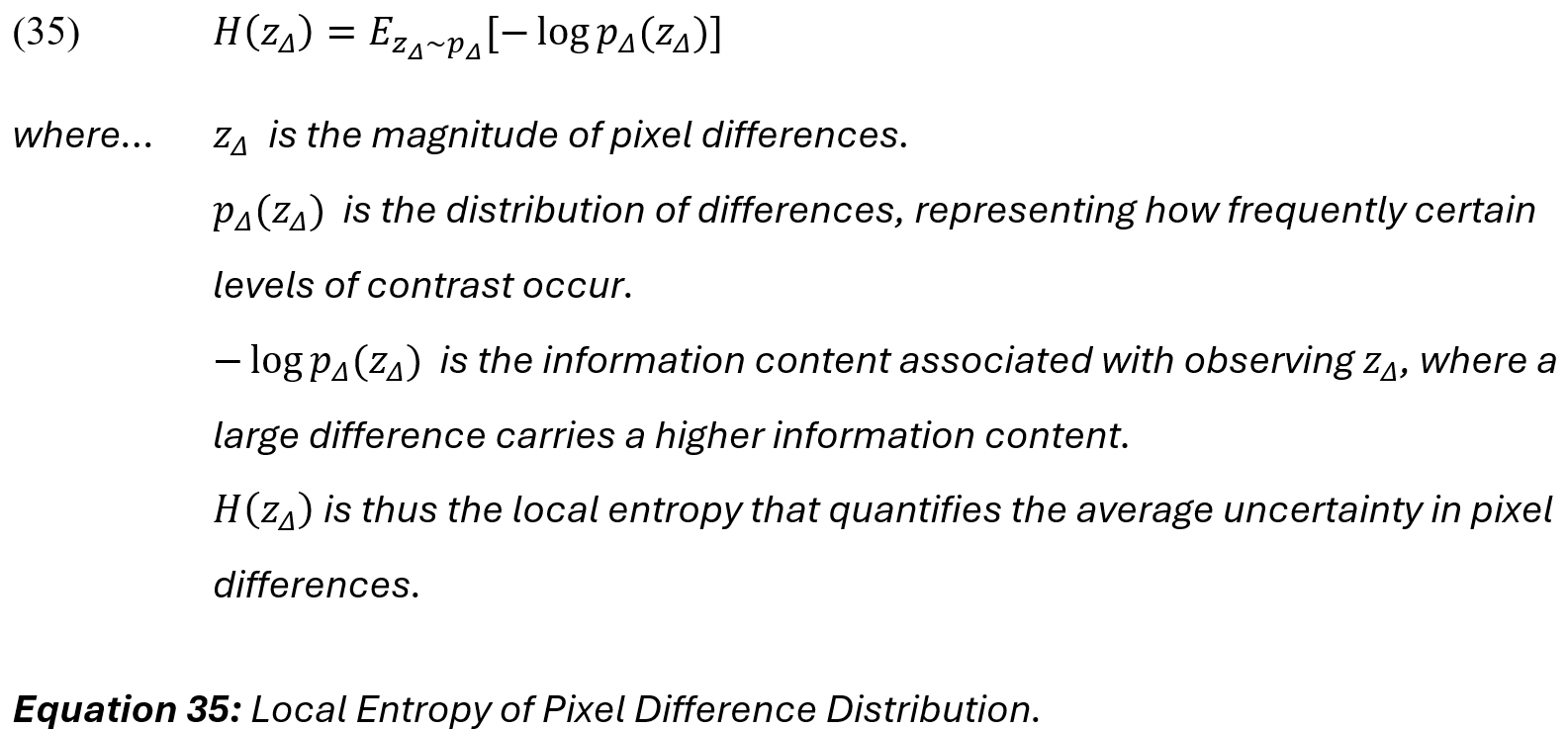
Therefore, the final metric to express discrete local entropy of pixel differences is:

In natural images, [p_delta (z_delta)] often shows a Laplacian-like distribution characterised by a peak near zero, reflecting small differences in smooth areas, and heavier tails, capturing larger differences corresponding to edges (Hyun jin Park & Lee, 2004). Hence, we can use equation (36) and knowledge of ‘real’ image distributions to quantify how ‘natural,’ or Laplacian-like, the local variations in an image are.
In Figure 6, we visualise the entropy distribution of pixel differences and observe a Laplacian-like shape in low- to mid-range differences and a second tail peak at [p_delta (z_delta)] = 250 , indicating deviations at higher pixel differences near the upper intensity limit. This result indicates that while the image largely follows a Laplacian-like distribution, there may be strong structural edges and/or generative artefacts present – which aligns with observations from our qualitative inspection.

If present, checkerboarding would introduce unnatural periodic patterns that alter [p_delta (z_delta)], manifesting abnormal peaks in the pixel difference distribution or inflated local entropies in otherwise uniform regions. In this case, the observed distributions do not indicate strong periodic artefacts, suggesting that the local variations remain largely natural.
This result aligns with theoretical expectations as, compared to GANs and DCNNs, diffusion approaches are less likely to suffer from checkerboarding precisely because their generative method relies on iterative denoising steps and score estimation, rather than convolution operations. Of course, checkerboarding can still be introduced into some diffusion approaches, such as latent diffusion models (LDMs), where we operate in a compressed latent space and upsample to reconstruct the final image. However, checkerboarding is only one of several types of artefacts that may occur. In Figure 5b-d, we incorporate checks for noise residue, blurring, and colour inconsistencies, respectively. To prevent scope creep, we will keep the descriptions of these next artefacts, our detection approaches, and results discussion relatively brief.
Figure 5b depicts an example of a noise residue analysis. Noise residue represents pixel-level random variations and refers to the remaining noise patterns in an image after applying a denoising process. As we have shown, noise addition and removal are instrumental to diffusion processes, but imperfect removal leads to residual noise, manifesting as subtle graininess or patterned distortions in the final output. The mean noise residue is calculated as the mean absolute difference between the original image [I] and its denoised version
[I_hat]. Higher values indicate more residual noise (i.e., incomplete denoising) and lower values indicate better noise suppression.
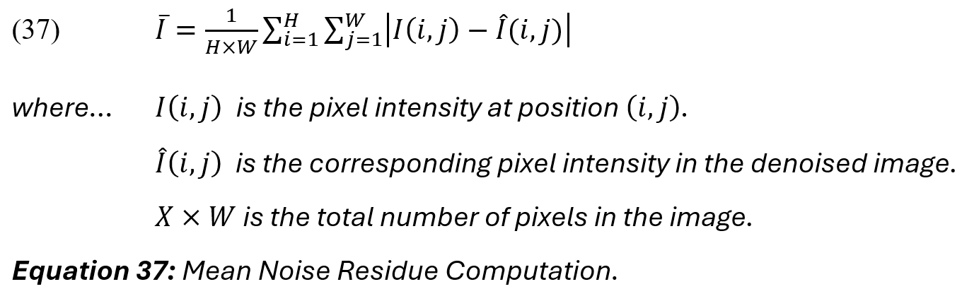
Our analysis shows a mean noise residue of ( [I_bar] = 83.97), indicating structured, non-random noise patterns typical of generative artefacts. This structured noise suggests incomplete denoising or upsampling-related artefacts, particularly in uniform regions, where the residual noise imperfections are the strongest.
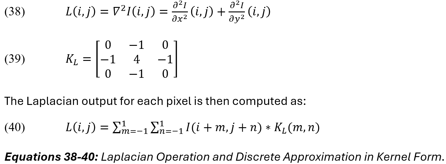
Figure 5c shows the Laplacian filter output, highlighting edges. Blurring refers to the loss of sharpness and fine details. In diffusion-based processes, rapid or incomplete denoising steps can smooth important structural features, leading to blurred edges and texture loss. Diffusion-based methods can introduce blurring when rapid or incomplete denoising over-smooths structural features, leading to blurry edges and/or losses of texture.
A Laplacian filter detects blurring by measuring the second-order derivatives of the image and, in doing so, highlights regions of rapid intensity changes, such as images, which are diminished when blurring occurs. Below is the Laplacian operation and a common discrete 3×3 approximation in kernel form:
The variance of the Laplacian is computed as a quantitative sharpness metric, where a higher variance indicates sharper images that have well-defined edges, and lower variance indicates blurring, where hard lines and edges are less pronounced:
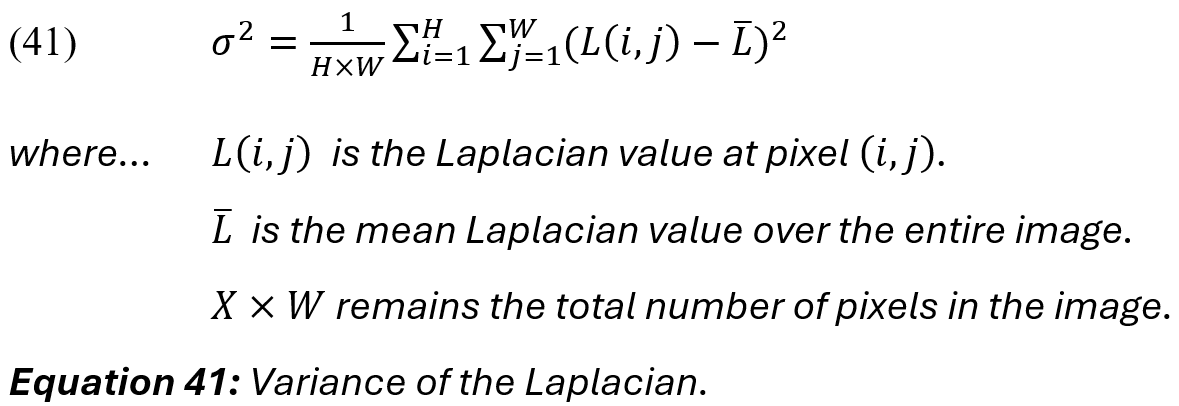
Our analysis shows a moderate variance value of ([sigma_sq] = 0.0183), which indicates some softness or mild blurring. The visual output of Figure 5c suggests that blurring is particularly visible in parts of the background and facial details. Foreground details like the old man’s hand and suit texture show more defined edges (i.e., less blurring) in these areas. This result is consistent with typical generative outputs, where moderate levels of blurring occur due to the unintentional replication of depth-of-field or focal emphasis effects, or as a consequence of using fewer diffusion steps [114].
Figure 5d depicts an example of a colour inconsistency analysis, where the differences between colour channels Red-Green (RG), Red-Blue (RB), and Green-Blue (GB) highlight areas of potential inconsistencies. To quantify color inconsistencies between channels, we computed the mean absolute difference [bar(delta_c1*c2)] between pixel intensities of the corresponding RGB channels:
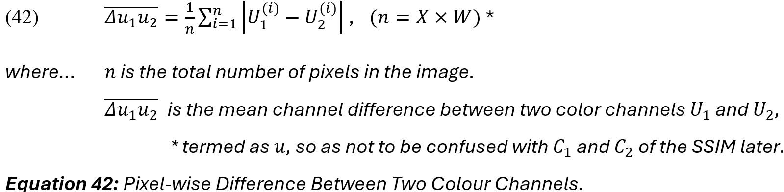
Our analysis shows a mean RG-difference of ( [bar(delta_RG)] = 54.19), a mean RB-difference of (
[bar(delta_RB)] = 84.12), and a mean GB-difference of (
[bar(delta_GB)] = 89.16). These results suggests that blue tones are less consistently aligned with other channels. The suit and skin tones show mild inconsistency, but are slight in comparison to the illumination issues present. In particular, the glass windows and floor reflections show noticeable channel differences, and is consistent with a qualitative observation of the windows and floors in Figure 4, where the colour tone variations in the scene’s lighting appear unnatural. Lighting inconsistencies are typical of generative models where we attempt to approximate global illumination without strict color consistency restraints.
For our final section of this example analysis, we move from artefacts to warping. Figure 5e shows a gradient magnitude map, which depicts spatial distortions and structural inconsistencies related to warping. The gradient magnitude measures the rate of intensity change at each pixel in an image. For an image [I(i, j)], the gradient can be expressed as partial derivatives in the horizontal x and vertical y directions:
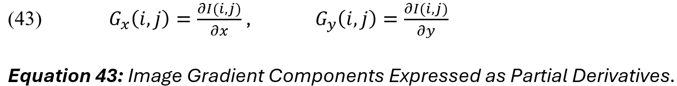
The gradient magnitude at each pixel (i, j) is given by the Euclidean norm of the gradient components. Recalling that images are discrete, we can approximate [G_x] and
[G_y] using convolutional kernels, like our aforementioned Sobel operator [20]:
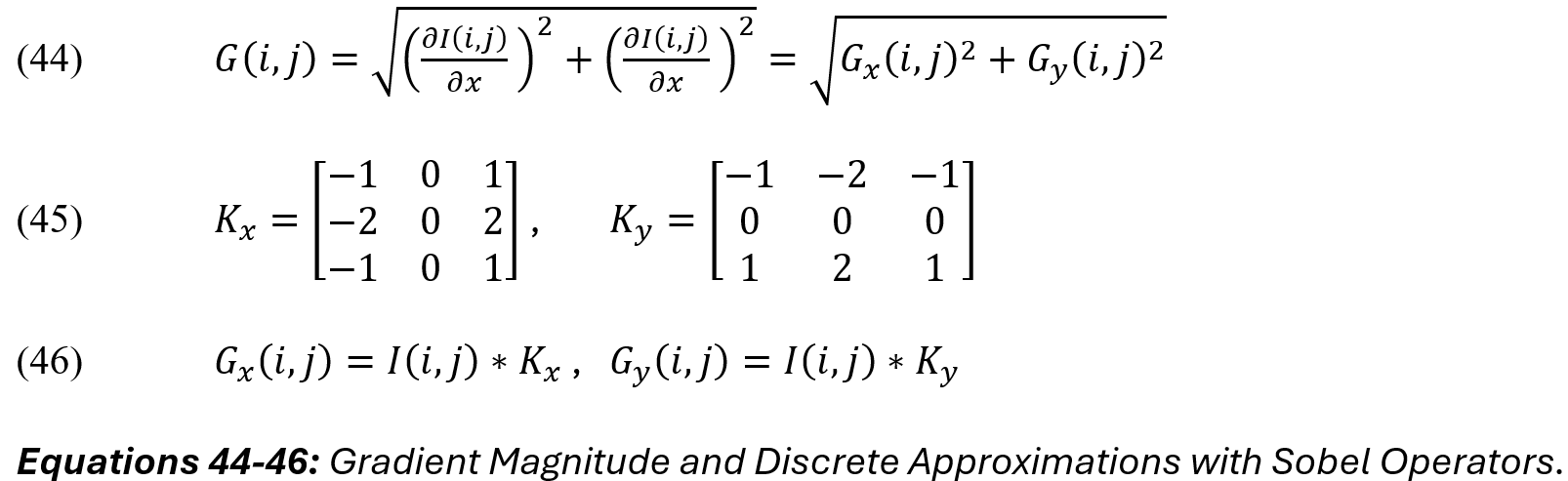
We then use the mean gradient magnitude to summarise the overall edge strength and detect potential warping, where higher mean values indicate strong structural transitions or potential warping in areas where abrupt changes should not exist:

Our analysis shows a mean gradient magnitude of ( [G_bar] = 993.98). High-gradient areas corresponding to brightness on the heatmap appear around the edges of the subject’s face and hand, background pillars, chandeliers, and window frames, suggesting largely strong structural definition in those areas. The background crowd shows moderate gradient variation, particularly where faces and body outlines do not align perfectly.
For more advanced, detailed information on spatial distortions and methods of detection, we recommend further reading:
- Principles of digital image forensics [115].
- Challenges in generating accurate projective geometry [114].
- Distortions relating to positional encoding [116].
We will now look at temporal coherence in video generation to better understand how temporal distortions are presented and detected.
Temporal Distortions
Temporal distortions represent another class of coherence challenges which result from introducing a temporal component into a generative task. In video generation, temporal distortions are inconsistencies between consecutive frames in video sequences that, when present, can disrupt the flow of motion and break the perception of continuity. Unlike spatial distortions which affect individual frames, temporal distortions impact how frames transition over time.
Common temporal distortions include events like flickering, jittering, ghosting, temporal incoherence, and temporal warping. Table 1 outlines common temporal distortion types, their causes, detection methods, high-level guidance for results interpretation, and key references. To maintain a narrow scope, we will examine only temporal incoherence in detail.
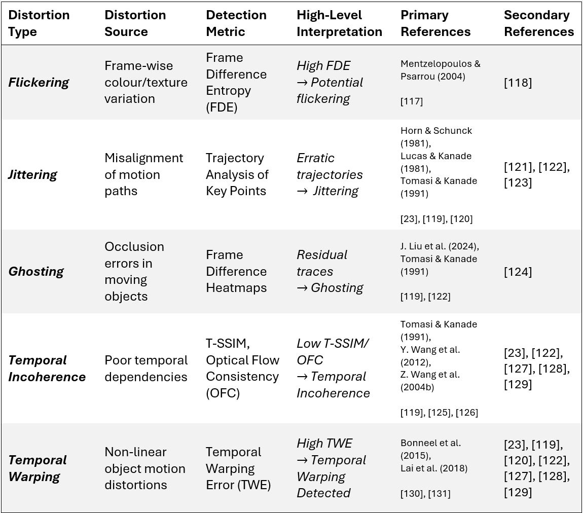
Temporal incoherence refers to missing or inconsistent temporal dependencies between frames, resulting in disjointed motion or abrupt changes in a subject or object’s position. Unlike flickering (i.e., frame-wise colour or texture fluctuations) or ghosting (i.e., occlusion errors, such as visual traces), temporal incoherence can be understood as a global video property.
For example, in one frame a person’s leg appears to be mid-stride, then in the next, it appears suddenly extended forward, skipping intermediate movement and giving the impression that frames might have been reordered or lost. This makes the video “temporally incoherent,” (i.e., the video’s global temporal structure is adversely affected by missing or inconsistent temporal dependencies), and so, while the person’s leg positions within static frames may appear natural, their motion does not once the frames are stitched together.
One way to measure temporal incoherence is via the Temporal Structural Similarity Index (T-SSIM) [126]. T-SSIM extends the traditional SSIM metric [125] to temporal sequences, measuring frame-to-frame structural consistency. Unlike traditional measures, such as Mean Squared Error (MSE) or Peak Signal-to-Noise Ratio (PSNR), which only capture pixel-wise differences, SSIM evaluates images based on structural information, offering a more robust metric for image quality:

The three components of the SSIM are:

Other works, such as Tomasi and Kanade’s optical flow measurement [119] and Wang et al.’s extension of the SSIM framework [126] demonstrate that low T-SSIM and OFC scores [see Table 1] correlate strongly with temporal incoherence. As Wang et al. explain in their formulation of T-SSIM, natural videos can be represented as pixels arranged along two spatial axes (x, y) and one temporal axis t, i.e., I(x, y, t). Given that pixels exhibit strong dependencies across both spatial and temporal domains, they propose a method for evaluating structural similarity for patches along the I(x, t) plane and I(y, t) plane in the same manner as in the I(x, y) spatial dimension. Recent contributions by Amin et al. [127] and Dosovitskiy et al. [129] further emphasise the need for motion-aware architectures to mitigate temporal distortions.
Block-based Approaches to Spatial and Temporal Coherence
Block-based approaches have been developed upon since the 1950s, though previously, they were largely used in the context of data compression and encoding [132], [133]. However, more recently they have been successfully adapted within state-of-the-art generative video frameworks.
As previously described, blocks are used to break video sequences into manageable, coherent units that ensure spatio-temporal coherence. These units represent subsets of frames that capture both spatial dependencies within frames, and temporal dependencies across frames. Processing videos in blocks allows models to effectively handle complex motion while maintaining local and global consistency.
Each block maintains spatial coherence by treating consecutive frames as part of a ‘single coherent unit’. Similarly, each block maintains temporal coherence by modelling frame sequences as continuous motion units. Transformer-based methods, RNNs, U-Nets, or even convolutional layers can be used to capture spatial and temporal dependencies and ensure smooth transitions in object motion and scene changes. Processing frames in this way helps the model synchronise object positions, reducing the likelihood of spatial distortions throughout the block, and prevent disjointed motion patterns at block boundaries. For instance, in Vision Transformer (ViT) and Diffusion Transformer (DiT) architectures, temporal attention mechanisms within each block help the model recognise long-range motion patterns and ensure consistent object trajectories across frames, while spatial attention mechanisms within each block enable the model to focus on salient regions and ensure that key objects are rendered consistently across frames [72], [134].
Often, the challenge is not in deciding whether to implement blocks but rather, how to architect a set of neural networks that can effectively generate high-fidelity video and control for spatial and temporal dependencies, without biasing or overly constraining the system. Thus, the notion of ‘ideal’ system architectures leads us to state-of-the-art methods for video generation.
7. State of the Art Models and Methods
Recent advancements in video generation have focused on striking a balance between spatial coherence and temporal continuity, two essential characteristics for generating high-quality, realistic videos. Sora is a state-of-the-art text-to-video generative AI model released by OpenAI in February 2024 [135]. In some contexts, and to OpenAI themselves, Sora also represents a world simulation model on the pathway to Artificial General Intelligence (AGI)[136]. However, for our specific context, we will consider it a large vision model (LVM) and a multimodal latent diffusion model (LDM) that uses a transformer-based architectures for block-based processing and video generation. For reasons of scope, we focus only on Sora’s design in this section, but in our evaluation, we provide a high-level overview of how this model’s hybrid architecture maintains quality, performance, and balance to achieve state-of-the-art results in video generation.
In Sora’s diffusion transformer architecture, spacetime latent patches serve as fundamental building blocks, and so we first compress raw videos into a latent spacetime representation and decompose this into spacetime patches. This approach to latent compression is based on Vector Quantised-VAE (VQ-VAE) methods [137], [138], allowing Sora to encapsulates both visual appearance and motion dynamics over short intervals. According to OpenAI, it is the same recaptioning technique used by DALL-E 3 to generate highly descriptive captions from visual training data [108], [139], [140], [141]. Following this, a ViT splits an image into fixed-size patches, linearly embeds each one, adds positional embeddings, and feeds the resulting sequence of vectors to a standard transformer encoder [2], [3].
In summary, the objectives of the first and second steps are to compress high-dimensional video data into a manageable latent space, then break these representations down into spacetime patches. To do this, input video sequences are encoded into a latent spacetime representation using a pretrained encoder. The latent space retains critical visual appearance and motion dynamics while significantly reducing dimensionality, improving computational efficiency. Once the latent spacetime volume is decomposed into patches, each patch represents short temporal intervals and spatial details. These patches serve as the fundamental units of generation, functioning similarly to word tokens in large language models, providing detailed visual phrases used to construct coherent video sequences
According to our findings, traditional diffusion models have mainly leveraged RNNs or convolutional U-Nets that include downsampling and upsampling blocks for the denoising network backbone [34], [59]. But more recent studies have shown that this not expressly necessary for good performance [2], [3], [5], [134]. Instead, Sora uses a DiT architecture to model spatio-temporal correlations by applying transformers to the latent space. Here, we use self-attention mechanisms to capture global temporal dynamics and spatial coherence. Temporal attention layers are added to model long-range dependencies across frames, and each transformer layer operates on the latent patches for parallel processing and scalability.
Then, we commence the diffusion process (i.e., latent denoising), where our objective is to generate high-quality video sequences through iterative denoising in the latent space. Though not discussed in a latent setting, the diffusion process mirrors diffusion as it is described in Section 5. As usual, we start with Gaussian noise in the latent space, iteratively refine the latent representation using a reverse diffusion process to recover the spatial structure and temporal consistency of the video.
After conducting forward and reverse (generative) diffusion processes, we use Temporal Super-Resolution (TSR) [not discussed in this review] to increase temporal resolution by interpolating additional frames. Effectively, TSR modules are applied to interpolate between generated frames, ensuring smooth motion trajectories and addressing temporal drift. Similarly, we use Spatial Super-Resolution (SSR) [not discussed in this review] to upscale latent frames and target spatial resolution. According to Liu et al., classifier-free guidance is used during training to help maintain structural details and lighting consistency [2]. Then, we introduce a correction mechanism for temporal drift to prevent incoherence during generation. On this point, we can expound:
We have already discussed how block-based generation ensures spatio-temporal consistency. In an orthogonal approach, each block is processed such that the generated frames are not only consistent over time, but also realistic at each time point. Here, orthogonality implies that spatial coherence and temporal continuity are treated as complementary, yet independent objectives. This separation allows the model to focus on generating structurally sound frames without sacrificing temporal coherence across the sequence.
In contrast, methods relying on continuous prediction, where each frame is generated based on preceding frames, risk overemphasising temporal continuity at the expense of spatial consistency. Specifically, a predictor may prioritise smooth transitions between frames, potentially producing frames that are temporally aligned but visually distorted, or less realistic when observed independently. Continuous prediction methods can achieve temporal coherence, but often fail to maintain spatial details (e.g., object boundaries, textures, or lighting conditions).
It is also important to note that orthogonality in this context refers to the independent treatment of spatial and temporal objectives within the architecture, rather than implying a specific number of neural networks. Similarly, continuous prediction methods may employ single or multi-component architectures, depending on the complexity of temporal modelling required.
Sora addresses these challenges by combining block-based generation with continuous prediction by employing a correction mechanism to prevent temporal drift. That is, if the generation process begins to diverge – e.g., if the model starts prioritising motion dynamics over the fidelity of individual frames – then the system recalibrates, effectively “knocking back” the divergence. This correction ensures that temporal dynamics do not overpower the spatial integrity of the generated frames.
While we have already described the benefit of this correction in terms of blocks, in summary – if the model starts prioritising motion dynamics over frame fidelity, a correction mechanism recalibrates the process, essentially “knocking back” any divergences and ensuring that temporal dynamics do not overpower spatial integrity. Finally, we decode the latent representations into high-fidelity video sequences. To do this, the refined latent frames are passed through a decoder and converted back to pixel-space videos. The final output is a state-of-the-art generated video that exhibits both spatial coherence within frames and temporal continuity across frames.
8. Conclusion and Open Challenges
As we’ve seen, video generation has evolved rapidly to meet the demands of a wide and enthusiastic audience. Building upon the foundations laid in this literature review, it is clear that while significant strides have been made in deep learning-based video generation, several open challenges persist. These challenges highlight the gaps in current methodologies and present exciting opportunities for future research. The following discussion outlines key areas where further exploration could push the boundaries of what is currently achievable.
Spatial Control of Object Trajectories
One [of many] under-investigated areas in video generation is spatial control of object trajectories. Although models like Sora achieve impressive spatial and temporal coherence, they often lack explicit control mechanisms to govern how objects move and interact within the spatial domain over time. Future research could explore:
- Trajectory-guided Generation:
Novel approaches like TrailBlazer [142] provide a glimpse into tools that incorporate trajectory-based conditioning during generation and allow users to specify motion paths for dynamic objects. Thus, one valuable research route would be to build upon a novel approach, such as TrailBlazer, with the aim of extending it into a general framework for addressing trajectory-guided video generation. - Scene-aware Spatial Control:
Scene decomposition and contextual encoding offer another promising research direction. Developing models capable of understanding and maintaining spatial relationships between multiple moving entities and static background elements is necessary for generative video tasks aspiring to replicate realism.
The ability to break down scenes into foreground and background layers can allow for more effective modelling of object interactions with static elements [6], [21], [143]. Additionally, integrating context-aware attention mechanisms would enable models to dynamically focus on relevant areas, based on object interactions. Together, these approaches could enhance the contextual consistency of generated videos, thus allowing more realistic movements and interactions in generated scenes.
Conclusion
This literature review has sought to position deep learning-based video generation as a dynamic and rapidly evolving field at a unique intersection of domains, though predominantely computer vision and computer graphics. We began by examining the shift from Generative Adversarial Networks (GANs) to the more robust and stable diffusion-based methods that now dominate in state-of-the-art generative image and video tasks, reflecting an increased preference for architectures capable of balancing robustness, stability, and fidelity.
Our exploration then turned to detailing the mechanics of diffusion models, which form the backbone of many state-of-the-art approaches. A comprehensive analysis of spatial and temporal coherence followed, highlighting the role of block-based architectures in addressing related distortions. We concluded this technical journey with an overview of Sora, a state-of-the-art model that exemplifies how hybrid architectures are better able to navigate spatio-temporal complexities to create realistic video sequences.
While these advancements are significant, several open challenges remain. Of particular interest is the need for enhanced control over object trajectories, scene-aware spatial dynamics, and semantic consistency. In our closing thoughts, we identify trajectory-guided generation, scene decomposition, and context-aware attention mechanisms as promising directions for future theoretical and practical investigation. By addressing some of these challenges, researchers could test the limits of controllable, contextually accurate, and interactive generative systems, capable of producing realistic video content for diverse applications. Looking ahead, addressing these challenges will be critical in narrowing the gap between the current capabilities of generative models and their practical deployment. As this technology continues to evolve, emphasis on explicit control mechanisms, advanced spatial reasoning, and semantic awareness will be key to realising their full potential. However, these technical achievements must also be accompanied by closer attention to social and legal frameworks that promote responsible deployment to ensuring that generative technologies are developed and used ethically and transparently. Only by striving for inclusion alongside technical and creative perfection can the field realise its full potential, offering not just technical breakthroughs but also trustworthy outcomes that benefit society at large.
References
[1] F. Bao et al., “Vidu: a Highly Consistent, Dynamic and Skilled Text-to-Video Generator with Diffusion Models,” 2024. [Online]. Available: https://arxiv.org/abs/2405.04233
[2] Y. Liu et al., “Sora: A Review on Background, Technology, Limitations, and Opportunities of Large Vision Models,” 2024. [Online]. Available: https://arxiv.org/abs/2402.17177
[3] F. Bao et al., “All are Worth Words: A ViT Backbone for Diffusion Models,” 2023. [Online]. Available: https://arxiv.org/abs/2209.12152
[4] D. H. Ballard and R. Zhang, “The Hierarchical Evolution in Human Vision Modeling,” Top Cogn Sci, vol. 13, no. 2, pp. 309–328, 2021, doi: https://doi.org/10.1111/tops.12527.
[5] F. Bao et al., “One Transformer Fits All Distributions in Multi-Modal Diffusion at Scale,” 2023. [Online]. Available: https://arxiv.org/abs/2303.06555
[6] M. Y. Yang, B. Rosenhahn, and V. Murino, “Chapter 1 – Introduction to Multimodal Scene Understanding,” in Multimodal Scene Understanding, M. Y. Yang, B. Rosenhahn, and V. Murino, Eds., Academic Press, 2019, pp. 1–7. doi: https://doi.org/10.1016/B978-0-12-817358-9.00007-X.
[7] R. S. Sutton and A. G. Barto, “Reinforcement Learning: An Introduction,” 2nd ed., Cambridge, Massachusetts; London, England: MIT Press, 2018, ch. 1: Introduction, pp. 1–13. [Online]. Available: http://incomplete-url-if-known
[8] J. Sohl-Dickstein, E. Weiss, N. Maheswaranathan, and S. Ganguli, “Deep Unsupervised Learning using Nonequilibrium Thermodynamics,” in Proceedings of the 32nd International Conference on Machine Learning, F. Bach and D. Blei, Eds., in Proceedings of Machine Learning Research, vol. 37. Lille, France: PMLR, Oct. 2015, pp. 2256–2265. [Online]. Available: https://proceedings.mlr.press/v37/sohl-dickstein15.html
[9] NVIDIA Corporation, “CUDA C++ Programming Guide,” Jan. 24, 2025. Accessed: Jan. 27, 2025. [Online]. Available: https://docs.nvidia.com/cuda/pdf/CUDA_C_Programming_Guide.pdf
[10] N. P. Jouppi et al., “In-Datacenter Performance Analysis of a Tensor Processing Unit,” 2017. [Online]. Available: https://arxiv.org/abs/1704.04760
[11] M. Abadi et al., “TensorFlow: Large-Scale Machine Learning on Heterogeneous Distributed Systems,” Mar. 2016, doi: 10.48550/arXiv.1603.04467.
[12] A. Paszke et al., PyTorch: An Imperative Style, High-Performance Deep Learning Library. 2019. doi: 10.48550/arXiv.1912.01703.
[13] R. Frostig, M. Johnson, and C. Leary, “Compiling machine learning programs via high-level tracing,” 2018. [Online]. Available: https://mlsys.org/Conferences/doc/2018/146.pdf
[14] T. J. Sejnowski, The Deep Learning Revolution. The MIT Press, 2018. doi: 10.7551/mitpress/11474.001.0001.
[15] L. Roberts, Machine Perception of Three-Dimensional Solids. 1963.
[16] D. Marr, H. K. Nishihara, and S. Brenner, “Representation and recognition of the spatial organization of three-dimensional shapes,” Proc R Soc Lond B Biol Sci, vol. 200, no. 1140, pp. 269–294, 1978, doi: 10.1098/rspb.1978.0020.
[17] D. Marr and S. Brenner, “Early processing of visual information,” Philosophical Transactions of the Royal Society of London. B, Biological Sciences, vol. 275, no. 942, pp. 483–519, 1976, doi: 10.1098/rstb.1976.0090.
[18] D. Marr, E. Hildreth, and S. Brenner, “Theory of edge detection,” Proc R Soc Lond B Biol Sci, vol. 207, no. 1167, pp. 187–217, 1980, doi: 10.1098/rspb.1980.0020.
[19] P.-E. Danielsson and O. Seger, “Generalized and Separable Sobel Operators,” 1990. [Online]. Available: https://api.semanticscholar.org/CorpusID:116392105
[20] I. Sobel and G. Feldman, “A 3×3 Isotropic Gradient Operator for Image Processing,” 1968. Accessed: Jan. 22, 2025. [Online]. Available: https://www.researchgate.net/publication/285159837_A_33_isotropic_gradient_operator_for_image_processing
[21] H. G. Barrow and J. M. Tenenbaum, “Recovering Intrinsic Scene Characteristics from Images,” in Computer Vision Systems, Digital Access., A. Hanson and E. Riseman, Eds., New York: Academic Press (1978), 1978, pp. 3–26. Accessed: Jan. 24, 2025. [Online]. Available: https://www.researchgate.net/publication/52006559_Computer_Vision_Systems
[22] J. M. Tenenbaum and H. G. Barrow, “Experiments in interpretation-guided segmentation,” Artif Intell, vol. 8, no. 3, pp. 241–274, 1977, doi: https://doi.org/10.1016/0004-3702(77)90031-5.
[23] B. K. P. Horn and B. G. Schunck, “Determining optical flow,” Artif Intell, vol. 17, no. 1, pp. 185–203, 1981, doi: https://doi.org/10.1016/0004-3702(81)90024-2.
[24] R. Woodham, “A Cooperative Algorithm for Determining Surface Orientation from a Single View.,” in Proc. 5th Int. Joint Conf. Artificial Intell., Jan. 1977, pp. 635–641.
[25] J. D. Mollon, “‘… On the Basis of Velocity Clues Alone’: Some Perceptual Themes 1946–1996,” The Quarterly Journal of Experimental Psychology Section A, vol. 50, no. 4, pp. 859–882, 1997, doi: 10.1080/713755736.
[26] J. Jing, S. Liu, G. Wang, W. Zhang, and C. Sun, “Recent advances on image edge detection: A comprehensive review,” Neurocomputing, vol. 503, pp. 259–271, 2022, doi: https://doi.org/10.1016/j.neucom.2022.06.083.
[27] O. A. Zuniga and R. M. Haralick, “Integrated Directional Derivative Gradient Operator,” IEEE Trans Syst Man Cybern, vol. 17, no. 3, pp. 508–517, 1987, doi: 10.1109/TSMC.1987.4309068.
[28] D. Marr and S. Brenner, “Analysis of occluding contour,” Proc R Soc Lond B Biol Sci, vol. 197, no. 1129, pp. 441–475, 1977, doi: 10.1098/rspb.1977.0080.
[29] J. Canny, “A Computational Approach to Edge Detection,” IEEE Trans Pattern Anal Mach Intell, vol. PAMI-8, no. 6, pp. 679–698, 1986, doi: 10.1109/TPAMI.1986.4767851.
[30] D. R. Martin, C. C. Fowlkes, and J. Malik, “Learning to detect natural image boundaries using local brightness, color, and texture cues,” IEEE Trans Pattern Anal Mach Intell, vol. 26, no. 5, pp. 530–549, 2004, doi: 10.1109/TPAMI.2004.1273918.
[31] S. Xie and Z. Tu, “Holistically-Nested Edge Detection,” in Proceedings of the IEEE International Conference on Computer Vision (ICCV), Dec. 2015.
[32] D. P. Kingma and M. Welling, “Auto-Encoding Variational Bayes,” 2022. [Online]. Available: https://arxiv.org/abs/1312.6114
[33] K. Simonyan and A. Zisserman, “Very Deep Convolutional Networks for Large-Scale Image Recognition,” 2015. [Online]. Available: https://arxiv.org/abs/1409.1556
[34] K. He, X. Zhang, S. Ren, and J. Sun, “Deep Residual Learning for Image Recognition,” 2015. [Online]. Available: https://arxiv.org/abs/1512.03385
[35] J. Yang, B. Price, S. Cohen, H. Lee, and M.-H. Yang, “Object Contour Detection With a Fully Convolutional Encoder-Decoder Network,” in Proceedings of the IEEE Conference on Computer Vision and Pattern Recognition (CVPR), Jun. 2016.
[36] Y. Liu, M.-M. Cheng, X. Hu, K. Wang, and X. Bai, “Richer Convolutional Features for Edge Detection,” in Proceedings of the IEEE Conference on Computer Vision and Pattern Recognition (CVPR), Jul. 2017.
[37] R. Deng, C. Shen, S. Liu, H. Wang, and X. Liu, “Learning to Predict Crisp Boundaries,” in Proceedings of the European Conference on Computer Vision (ECCV), Sep. 2018.
[38] M. Pu, Y. Huang, Y. Liu, Q. Guan, and H. Ling, “EDTER: Edge Detection With Transformer,” in Proceedings of the IEEE/CVF Conference on Computer Vision and Pattern Recognition (CVPR), Jun. 2022, pp. 1402–1412.
[39] C. Lamotte, “Discovering Animation Manuals: Their Place and Role in the History of Animation,” Animation : an interdisciplinary journal, vol. 17, no. 1, pp. 127–143, 2022, doi: 10.1177/17468477221080112.
[40] E. Catmull, “The problems of computer-assisted animation,” in Proceedings of the 5th Annual Conference on Computer Graphics and Interactive Techniques, in SIGGRAPH ’78. New York, NY, USA: Association for Computing Machinery, 1978, pp. 348–353. doi: 10.1145/800248.807414.
[41] D. Terzopoulos, J. Platt, A. Barr, and K. Fleischer, Elastically Deformable Models, vol. 21. 1987. doi: 10.1145/37402.37427.
[42] K. Perlin, “An image synthesizer,” in Proceedings of the 12th Annual Conference on Computer Graphics and Interactive Techniques, in SIGGRAPH ’85. New York, NY, USA: Association for Computing Machinery, 1985, pp. 287–296. doi: 10.1145/325334.325247.
[43] S. Liu, Z. Ren, S. Gupta, and S. Wang, “PhysGen: Rigid-Body Physics-Grounded Image-to-Video Generation,” 2024. [Online]. Available: https://arxiv.org/abs/2409.18964
[44] L. S. Aira, A. Montanaro, E. Aiello, D. Valsesia, and E. Magli, “MotionCraft: Physics-based Zero-Shot Video Generation,” 2024. [Online]. Available: https://arxiv.org/abs/2405.13557
[45] P. Perona and J. Malik, “Scale-space and edge detection using anisotropic diffusion,” IEEE Trans Pattern Anal Mach Intell, vol. 12, no. 7, pp. 629–639, 1990, doi: 10.1109/34.56205.
[46] B. D. O. Anderson, “Reverse-time diffusion equation models,” Stoch Process Their Appl, vol. 12, no. 3, pp. 313–326, May 1982, [Online]. Available: https://ideas.repec.org/a/eee/spapps/v12y1982i3p313-326.html
[47] T. Beier and S. Neely, “Feature-based image metamorphosis,” in Proceedings of the 19th Annual Conference on Computer Graphics and Interactive Techniques, in SIGGRAPH ’92. New York, NY, USA: Association for Computing Machinery, 1992, pp. 35–42. doi: 10.1145/133994.134003.
[48] M. Levoy and P. Hanrahan, “Light field rendering,” in Proceedings of the 23rd Annual Conference on Computer Graphics and Interactive Techniques, in SIGGRAPH ’96. New York, NY, USA: Association for Computing Machinery, 1996, pp. 31–42. doi: 10.1145/237170.237199.
[49] T. Whitted, “An improved illumination model for shaded display,” Commun. ACM, vol. 23, no. 6, pp. 343–349, Jun. 1980, doi: 10.1145/358876.358882.
[50] I. Carlbom and J. Paciorek, “Planar Geometric Projections and Viewing Transformations,” ACM Computing Surveys (CSUR), vol. 10, pp. 465–502, Dec. 1978, doi: 10.1145/356744.356750.
[51] M. Potmesil and I. Chakravarty, “A lens and aperture camera model for synthetic image generation,” in Proceedings of the 8th Annual Conference on Computer Graphics and Interactive Techniques, in SIGGRAPH ’81. New York, NY, USA: Association for Computing Machinery, 1981, pp. 297–305. doi: 10.1145/800224.806818.
[52] M. Potmesil and I. Chakravarty, “Synthetic Image Generation with a Lens and Aperture Camera Model,” ACM Trans. Graph., vol. 1, no. 2, pp. 85–108, Apr. 1982, doi: 10.1145/357299.357300.
[53] K. Park et al., “Nerfies: Deformable Neural Radiance Fields,” in Proceedings of the IEEE/CVF International Conference on Computer Vision (ICCV), Oct. 2021, pp. 5865–5874.
[54] K. Zhang, G. Riegler, N. Snavely, and V. Koltun, “NeRF++: Analyzing and Improving Neural Radiance Fields,” 2020. [Online]. Available: https://arxiv.org/abs/2010.07492
[55] K. Gao, Y. Gao, H. He, D. Lu, L. Xu, and J. Li, “NeRF: Neural Radiance Field in 3D Vision, A Comprehensive Review,” 2023. [Online]. Available: https://arxiv.org/abs/2210.00379
[56] E. Tabak and T. Cristina, “A Family of Nonparametric Density Estimation Algorithms,” Commun Pure Appl Math, vol. 66, Feb. 2013, doi: 10.1002/cpa.21423.
[57] E. Tabak and E. Vanden-Eijnden, “Density estimation by dual ascent of the log-likelihood,” Communications in Mathematical Sciences – COMMUN MATH SCI, vol. 8, Mar. 2010, doi: 10.4310/CMS.2010.v8.n1.a11.
[58] I. J. Goodfellow et al., “Generative Adversarial Networks,” 2014. [Online]. Available: https://arxiv.org/abs/1406.2661
[59] O. Ronneberger, P. Fischer, and T. Brox, “U-Net: Convolutional Networks for Biomedical Image Segmentation,” 2015. [Online]. Available: https://arxiv.org/abs/1505.04597
[60] A. Krizhevsky, I. Sutskever, and G. Hinton, “ImageNet Classification with Deep Convolutional Neural Networks,” Neural Information Processing Systems, vol. 25, Jan. 2012, doi: 10.1145/3065386.
[61] A. Radford, L. Metz, and S. Chintala, “Unsupervised Representation Learning with Deep Convolutional Generative Adversarial Networks,” 2016. [Online]. Available: https://arxiv.org/abs/1511.06434
[62] PyTorch, “DCGAN Tutorial – PyTorch,” 2024.
[63] S. Stabinger, D. Peer, and A. Rodríguez-Sánchez, “Arguments for the Unsuitability of Convolutional Neural Networks for Non–Local Tasks,” 2021. [Online]. Available: https://arxiv.org/abs/2102.11944
[64] Z. Wang and L. Wu, “Theoretical Analysis of Inductive Biases in Deep Convolutional Networks,” 2024. [Online]. Available: https://arxiv.org/abs/2305.08404
[65] A. Brock, J. Donahue, and K. Simonyan, “Large Scale GAN Training for High Fidelity Natural Image Synthesis,” 2019. [Online]. Available: https://arxiv.org/abs/1809.11096
[66] T. Karras, S. Laine, and T. Aila, “A Style-Based Generator Architecture for Generative Adversarial Networks,” 2019. [Online]. Available: https://arxiv.org/abs/1812.04948
[67] M. Kang, J. Shin, and J. Park, “StudioGAN: A Taxonomy and Benchmark of GANs for Image Synthesis,” 2023. [Online]. Available: https://arxiv.org/abs/2206.09479
[68] Z. Duan, M. Lu, J. Ma, Y. Huang, Z. Ma, and F. Zhu, “QARV: Quantization-Aware ResNet VAE for Lossy Image Compression,” IEEE Trans Pattern Anal Mach Intell, vol. 46, no. 1, pp. 436–450, Jan. 2024, doi: 10.1109/tpami.2023.3322904.
[69] J. Stastny, “VAE-ResNet18-PyTorch,” 2019. [Online]. Available: https://github.com/julianstastny/VAE-ResNet18-PyTorch
[70] A. Graikos, S. Yellapragada, and D. Samaras, “Conditional Generation from Unconditional Diffusion Models using Denoiser Representations,” 2023. [Online]. Available: https://arxiv.org/abs/2306.01900
[71] A. Vaswani et al., “Attention Is All You Need,” 2023. [Online]. Available: https://arxiv.org/abs/1706.03762
[72] A. Dosovitskiy et al., “An Image is Worth 16×16 Words: Transformers for Image Recognition at Scale,” 2021. [Online]. Available: https://arxiv.org/abs/2010.11929
[73] L. Mescheder, S. Nowozin, and A. Geiger, “The Numerics of GANs,” 2018. [Online]. Available: https://arxiv.org/abs/1705.10461
[74] I. Csiszár, “Information-type measures of difference of probability distributions and indirect observations,” Studia Scientiarum Mathematicarum Hungarica, vol. 2, pp. 299–318, 1967.
[75] S. M. Ali and S. D. Silvey, “A General Class of Coefficients of Divergence of One Distribution from Another,” Journal of the Royal Statistical Society: Series B (Methodological), vol. 28, no. 1, pp. 131–142, 1966.
[76] I. Csiszár, “Eine informationstheoretische Ungleichung und ihre Anwendung auf den Beweis der Ergodizität von Markoffschen Ketten,” Magyar Tudományos Akadémia Matematikai Kutató Intézetének Közleményei, vol. 8, no. 1–2, pp. 85–108, 1963.
[77] X. Nguyen, M. J. Wainwright, and M. I. Jordan, “Estimating divergence functionals and the likelihood ratio by convex risk minimization,” IEEE Trans Inf Theory, vol. 56, no. 11, pp. 5847–5861, Nov. 2010, doi: 10.1109/TIT.2010.2068870.
[78] M. Arjovsky, S. Chintala, and L. Bottou, “Wasserstein GAN,” 2017. [Online]. Available: https://arxiv.org/abs/1701.07875
[79] X. Mao, Q. Li, H. Xie, R. Y. K. Lau, Z. Wang, and S. P. Smolley, “Least Squares Generative Adversarial Networks,” in 2017 IEEE International Conference on Computer Vision (ICCV), 2017, pp. 2813–2821. doi: 10.1109/ICCV.2017.304.
[80] A. Sauer, D. Lorenz, A. Blattmann, and R. Rombach, “Adversarial Diffusion Distillation,” 2023. [Online]. Available: https://arxiv.org/abs/2311.17042
[81] A. Sauer, F. Boesel, T. Dockhorn, A. Blattmann, P. Esser, and R. Rombach, “Fast High-Resolution Image Synthesis with Latent Adversarial Diffusion Distillation,” 2024. [Online]. Available: https://arxiv.org/abs/2403.12015
[82] J. Ho, A. Jain, and P. Abbeel, “Denoising Diffusion Probabilistic Models,” 2020. [Online]. Available: https://arxiv.org/abs/2006.11239
[83] B. Kleijn, “Diffusion [Lecture 9 Notes],” Master of Artificial Intelligence, Victoria University of Wellington, Sep. 2024, Accessed: Oct. 04, 2024. [Online]. Available: https://ecs.wgtn.ac.nz/foswiki/pub/Courses/AIML425_2024T2/LectureSchedule/diffusion425.pdf
[84] B. D. O. Anderson, A. N. Bishop, P. Del Moral, and C. Palmier, “Backward Nonlinear Smoothing Diffusions,” Theory of Probability & Its Applications, vol. 66, no. 2, pp. 245–262, Jan. 2021, doi: 10.1137/s0040585x97t99037x.
[85] A. Hyvärinen, “Estimation of Non-Normalized Statistical Models by Score Matching.,” Journal of Machine Learning Research, vol. 6, pp. 695–709, Jan. 2005.
[86] Y. Song, J. Sohl-Dickstein, D. P. Kingma, A. Kumar, S. Ermon, and B. Poole, “Score-Based Generative Modeling through Stochastic Differential Equations,” 2021. [Online]. Available: https://arxiv.org/abs/2011.13456
[87] A. Hyvarinen, “Connections Between Score Matching, Contrastive Divergence, and Pseudolikelihood for Continuous-Valued Variables,” IEEE Trans Neural Netw, vol. 18, no. 5, pp. 1529–1531, 2007, doi: 10.1109/TNN.2007.895819.
[88] A. Hyvärinen, “Some extensions of score matching,” Comput Stat Data Anal, vol. 51, no. 5, pp. 2499–2512, 2007, doi: https://doi.org/10.1016/j.csda.2006.09.003.
[89] A. Hyvärinen, “Optimal Approximation of Signal Priors,” Neural Comput, vol. 20, no. 12, pp. 3087–3110, Dec. 2008, doi: 10.1162/neco.2008.10-06-384.
[90] E. L. Allgower and K. Georg, “Predictor-Corrector Methods Using Updating,” in Numerical Continuation Methods: An Introduction, E. L. Allgower and K. Georg, Eds., Berlin, Heidelberg: Springer Berlin Heidelberg, 1990, pp. 61–74. doi: 10.1007/978-3-642-61257-2_7.
[91] Y. Song and S. Ermon, “Generative Modeling by Estimating Gradients of the Data Distribution,” 2020. [Online]. Available: https://arxiv.org/abs/1907.05600
[92] M. S. Albergo and E. Vanden-Eijnden, “Building Normalizing Flows with Stochastic Interpolants,” 2023. [Online]. Available: https://arxiv.org/abs/2209.15571
[93] B. Kleijn, “Normalising Flows [Lecture 8 Notes],” Master of Artificial Intelligence, Victoria University of Wellington, Sep. 2024, Accessed: Oct. 06, 2024. [Online]. Available: https://ecs.wgtn.ac.nz/foswiki/pub/Courses/AIML425_2024T2/LectureSchedule/flows.pdf
[94] T. Karras, M. Aittala, T. Aila, and S. Laine, “Elucidating the Design Space of Diffusion-Based Generative Models,” 2022. [Online]. Available: https://arxiv.org/abs/2206.00364
[95] J. B. J. Fourier, G. Darboux, and et al., “Théorie analytique de la chaleur,” Didot Paris, vol. 504, 1822, doi: 10.1016/B978-044450871-3/50107-8.
[96] G. Hinton, O. Vinyals, and J. Dean, “Distilling the knowledge in a neural network,” arXiv preprint arXiv:1503.02531, 2015.
[97] T. Salimans and J. Ho, “Progressive Distillation for Fast Sampling of Diffusion Models,” 2022. [Online]. Available: https://arxiv.org/abs/2202.00512
[98] E. Keogh and A. Mueen, “Curse of Dimensionality,” in Encyclopedia of Machine Learning and Data Mining, C. Sammut and G. I. Webb, Eds., Boston, MA: Springer US, 2017, pp. 314–315. doi: 10.1007/978-1-4899-7687-1_192.
[99] L. P. Cinelli, E. A. Barros da Silva, S. L. Netto, and M. A. Marins, “Fundamentals of Statistical Inference,” Switzerland: Springer International Publishing AG, 2021, pp. 5–30. doi: 10.1007/978-3-030-70679-1_2.
[100] D. P. Kroese, R. Y. Rubinstein, D. P. Kroese, and R. Y. Rubinstein, “MARKOV CHAIN MONTE CARLO,” vol. 10, United States: John Wiley & Sons, Incorporated, 2016, pp. 187–220. doi: 10.1002/9781118631980.ch6.
[101] V. Wilhelm, M. Krüger, M. Fuchs, and F. Vogel, Evaluation of the probability current in the stochastic path integral formalism. 2024. doi: 10.48550/arXiv.2411.14004.
[102] Y. Song, J. Sohl-Dickstein, D. P. Kingma, A. Kumar, S. Ermon, and B. Poole, “Score-Based Generative Modeling through Stochastic Differential Equations,” Nov. 2020, [Online]. Available: http://arxiv.org/abs/2011.13456
[103] B. Øksendal, “Stochastic Differential Equations,” in Stochastic Differential Equations: An Introduction with Applications, B. Øksendal, Ed., Berlin, Heidelberg: Springer Berlin Heidelberg, 2003, pp. 65–84. doi: 10.1007/978-3-642-14394-6_5.
[104] B. Øksendal, “The Itô Formula and the Martingale Representation Theorem,” in Stochastic Differential Equations: An Introduction with Applications, B. Øksendal, Ed., Berlin, Heidelberg: Springer Berlin Heidelberg, 2003, pp. 43–63. doi: 10.1007/978-3-642-14394-6_4.
[105] B. Øksendal, “Diffusions: Basic Properties,” in Stochastic Differential Equations: An Introduction with Applications, B. Øksendal, Ed., Berlin, Heidelberg: Springer Berlin Heidelberg, 2003, pp. 115–140. doi: 10.1007/978-3-642-14394-6_7.
[106] J. Ho et al., “Imagen Video: High Definition Video Generation with Diffusion Models,” 2022. [Online]. Available: https://arxiv.org/abs/2210.02303
[107] R. T. Q. Chen, Y. Rubanova, J. Bettencourt, and D. Duvenaud, “Neural Ordinary Differential Equations,” Jun. 2018, [Online]. Available: http://arxiv.org/abs/1806.07366
[108] J. Betker et al., “Improving Image Generation with Better Captions,” OpenAI, Microsoft, 2023. [Online]. Available: https://api.semanticscholar.org/CorpusID:264403242
[109] B. Kleijn, “Convolutional Neural Networks: AIML425 [Lecture 5 Notes],” Master of Artificial Intelligence, Victoria University of Wellington, Aug. 2024, Accessed: Sep. 08, 2024. [Online]. Available: https://ecs.wgtn.ac.nz/foswiki/pub/Courses/AIML425_2024T2/LectureSchedule/lect5CNN.pdf
[110] E. O. Brigham and R. E. Morrow, “The fast Fourier transform,” IEEE Spectr, vol. 4, no. 12, pp. 63–70, 1967, doi: 10.1109/MSPEC.1967.5217220.
[111] Z. Wang, A. C. Bovik, H. R. Sheikh, and E. P. Simoncelli, “Image quality assessment: from error visibility to structural similarity,” IEEE Transactions on Image Processing, vol. 13, no. 4, pp. 600–612, 2004, doi: 10.1109/TIP.2003.819861.
[112] B. Kleijn, “Brief Review Probability Theory and Basic Information Theoric Quantities as Used in Deep Learning: AIML425 [Lecture 1 Notes],” Master of Artificial Intelligence, Victoria University of Wellington, pp. 16–20, Jul. 2024, Accessed: Jul. 18, 2024. [Online]. Available: https://ecs.wgtn.ac.nz/foswiki/pub/Courses/AIML425_2024T2/LectureSchedule/probability.pdf
[113] hyun jin Park and T.-W. Lee, Modeling Nonlinear Dependencies in Natural Images using Mixture of Laplacian Distribution. 2004.
[114] A. Sarkar, H. Mai, A. Mahapatra, S. Lazebnik, D. A. Forsyth, and A. Bhattad, “Shadows Don’t Lie and Lines Can’t Bend! Generative Models don’t know Projective Geometry…for now,” 2024. [Online]. Available: https://arxiv.org/abs/2311.17138
[115] H. Farid, “Digital Image Forensics,” 2009.
[116] J. Choi, J. Lee, Y. Jeong, and S. Yoon, “Toward Spatially Unbiased Generative Models,” 2021. [Online]. Available: https://arxiv.org/abs/2108.01285
[117] M. Mentzelopoulos and A. Psarrou, “Key-frame extraction algorithm using entropy difference,” in Proceedings of the 6th ACM SIGMM International Workshop on Multimedia Information Retrieval, in MIR ’04. New York, NY, USA: Association for Computing Machinery, 2004, pp. 39–45. doi: 10.1145/1026711.1026719.
[118] H. Wu et al., “DisCoVQA: Temporal Distortion-Content Transformers for Video Quality Assessment,” 2022. [Online]. Available: https://arxiv.org/abs/2206.09853
[119] C. Tomasi and T. Kanade, “Detection and Tracking of Point Features,” Pittsburgh, PA, 1991. [Online]. Available: https://www.ri.cmu.edu/pub_files/pub2/tomasi_c_1991_1/tomasi_c_1991_1.pdf
[120] B. D. Lucas and T. Kanade, “An Iterative Image Registration Technique with an Application to Stereo Vision,” in Proceedings of the 7th International Joint Conference on Artificial Intelligence, Vancouver, BC, Canada, 1981, pp. 674–679. [Online]. Available: https://ecommons.cornell.edu/bitstream/handle/1813/64117/81-1303.pdf
[121] H. Farid, “Image Forensics,” in Computer Vision, K. Ikeuchi, Ed., Springer Nature Switzerland AG, 2020. doi: 10.1007/978-3-030-03243-2_877-12.
[122] J. Liu, Y. Qu, Q. Yan, X. Zeng, L. Wang, and R. Liao, “Fréchet Video Motion Distance: A Metric for Evaluating Motion Consistency in Videos,” 2024. [Online]. Available: https://arxiv.org/abs/2407.16124
[123] T. Unterthiner, S. van Steenkiste, K. Kurach, R. Marinier, M. Michalski, and S. Gelly, “FVD: A New Metric for Video Generation,” in International Conference on Learning Representations (ICLR) Workshop, 2019. [Online]. Available: https://openreview.net/pdf?id=rylgEULtdN
[124] X. Li et al., “Sharp Multiple Instance Learning for DeepFake Video Detection,” in Proceedings of the 28th ACM International Conference on Multimedia, in MM ’20. New York, NY, USA: Association for Computing Machinery, 2020, pp. 1864–1872. doi: 10.1145/3394171.3414034.
[125] Z. Wang, A. C. Bovik, H. R. Sheikh, and E. P. Simoncelli, “Image quality assessment: from error visibility to structural similarity,” IEEE Transactions on Image Processing, vol. 13, no. 4, pp. 600–612, 2004, doi: 10.1109/TIP.2003.819861.
[126] Y. Wang, T. Jiang, S. Ma, and W. Gao, “Spatio-temporal ssim index for video quality assessment,” in 2012 Visual Communications and Image Processing, 2012, pp. 1–6. doi: 10.1109/VCIP.2012.6410779.
[127] M. A. Amin, Y. Hu, and J. Hu, “Analyzing temporal coherence for deepfake video detection,” Electronic Research Archive, vol. 32, no. 4, pp. 2621–2641, 2024, doi: 10.3934/era.2024119.
[128] E. Ilg, N. Mayer, T. Saikia, M. Keuper, A. Dosovitskiy, and T. Brox, “FlowNet 2.0: Evolution of Optical Flow Estimation with Deep Networks,” in Proceedings of the IEEE Conference on Computer Vision and Pattern Recognition (CVPR), 2017, pp. 2462–2470. [Online]. Available: https://openaccess.thecvf.com/content_cvpr_2017/html/Ilg_FlowNet_2.0_Evolution_CVPR_2017_paper.html
[129] A. Dosovitskiy et al., “FlowNet: Learning Optical Flow with Convolutional Networks,” in Proceedings of the IEEE International Conference on Computer Vision (ICCV), 2015, pp. 2758–2766. [Online]. Available: https://www.cv-foundation.org/openaccess/content_iccv_2015/papers/Dosovitskiy_FlowNet_Learning_Optical_ICCV_2015_paper.pdf
[130] N. Bonneel, J. Tompkin, K. Sunkavalli, D. Sun, S. Paris, and H. Pfister, “Blind video temporal consistency,” ACM Trans. Graph., vol. 34, no. 6, Nov. 2015, doi: 10.1145/2816795.2818107.
[131] W.-S. Lai, J.-B. Huang, O. Wang, E. Shechtman, E. Yumer, and M.-H. Yang, “Learning Blind Video Temporal Consistency,” 2018. [Online]. Available: https://arxiv.org/abs/1808.00449
[132] C. Reader, “History of Video Compression (Draft),” 2002. [Online]. Available: https://en.wikipedia.org/wiki/Motion_compensation?utm_source=chatgpt.com
[133] J. A. Roese and G. S. Robinson, “Combined Spatial and Temporal Coding of Digital Image Sequences,” in Efficient Transmission of Pictorial Information, in Proceedings of SPIE, vol. 66. 1975, pp. 15–20. doi: 10.1117/12.954858.
[134] W. Peebles and S. Xie, “Scalable Diffusion Models with Transformers,” in Proceedings of the IEEE/CVF International Conference on Computer Vision (ICCV), 2023, pp. 1–10. [Online]. Available: https://arxiv.org/abs/2212.09748
[135] OpenAI, “Sora System Card,” 2024. [Online]. Available: https://openai.com/index/sora-system-card/
[136] OpenAI, “Video Generation Models as World Simulators,” 2024. [Online]. Available: https://openai.com/index/video-generation-models-as-world-simulators/
[137] W. Yan, Y. Zhang, P. Abbeel, and A. Srinivas, “VideoGPT: Video Generation using VQ-VAE and Transformers,” 2021. [Online]. Available: https://arxiv.org/abs/2104.10157
[138] A. Razavi, A. van den Oord, and O. Vinyals, “Generating Diverse High-Fidelity Images with VQ-VAE-2,” 2019. [Online]. Available: https://arxiv.org/abs/1906.00446
[139] A. Ramesh, P. Dhariwal, A. Nichol, C. Chu, and M. Chen, “Hierarchical Text-Conditional Image Generation with CLIP Latents,” 2022. [Online]. Available: https://arxiv.org/abs/2204.06125
[140] A. Ramesh et al., “Zero-Shot Text-to-Image Generation,” 2021. [Online]. Available: https://arxiv.org/abs/2102.12092
[141] A. Radford et al., “Learning Transferable Visual Models From Natural Language Supervision,” 2021. [Online]. Available: https://arxiv.org/abs/2103.00020
[142] W.-D. K. Ma, J. P. Lewis, and W. B. Kleijn, “TrailBlazer: Trajectory Control for Diffusion-Based Video Generation,” arXiv preprint arXiv:2401.00896, 2024, [Online]. Available: https://hohonu-vicml.github.io/Trailblazer.Page/
[143] C. Vondrick, H. Pirsiavash, and A. Torralba, “Generating Videos with Scene Dynamics,” in Advances in Neural Information Processing Systems, D. Lee, M. Sugiyama, U. Luxburg, I. Guyon, and R. Garnett, Eds., Curran Associates, Inc., 2016. [Online]. Available: https://proceedings.neurips.cc/paper_files/paper/2016/file/04025959b191f8f9de3f924f0940515f-Paper.pdf
